- 投稿日:2019-05-27T23:58:56+09:00
DataFrame や Series内のデータ参照は「iat」で行おう
はじめに
こんにちは。
現在東京大学で主にシステムデザインを学んでいる学生です。
授業で少し大きめのデータを扱った際に普段より長い処理時間に苦労したので、その時に試したちょっとした高速化の工夫をご紹介したいと思います。用意したDataFrame
名前:Data
長さ:10**6
カラム:ITEM, NUM (適当に作った為、特に意味の無いデータです)>>> Data.head() ITEM NUM 0 02134 1 1 04137 1 2 03900 1 3 00792 1 4 03678 1 >>> print(len(Data)) 1000000メソッドごとの処理時間の比較
ただデータにアクセスするだけの処理を行い、掛かった時間を比較しています。
1. メソッドを用いない場合(カラム名、インデックスで直接指定)
t = time.time()
for i in range(len(Data)):
    Data['NUM'][i]
print(time.time()-t)
# 54.22648358345032
2.
.ilocを用いた場合t = time.time() for i in range(len(Data)): Data.iloc[i,1] print(time.time()-t) # 16.671371221542363.
.iatを用いた場合t = time.time() for i in range(len(Data)): Data.iat[i,1] print(time.time()-t) # 10.457467794418335結果
それぞれの処理時間をまとめると以下のようになりました。
メソッド データ数 処理時間(s) 無 10^6 54.23 iloc 10^6 16.67 iat 10^6 10.46 感想
10^6 程の大きさのデータに対してもこれだけの差が出るとは思っていなかった為、少々驚きました。
大きめのデータを扱う際にはPythonのライブラリのメソッドを積極的に活用していきたいと思います。
- 投稿日:2019-05-27T23:17:30+09:00
最新機械学習モデル HistGradientBoostingTreeの性能調査(LightGBMと比較検証)
Abstract
ヒストグラムベースのGradientBoostingTreeが追加されたので、系譜のLightGBMと比較した使用感を検証する。
今回はハイパーパラメータ探索のOptunaを使い、パラメータ探索時点から速度や精度を比較検証する。
最後にKaggleにSubmissionして、汎用性を確認する。Introduction
scikit-learn v0.21 で追加された HistGradientBoosting*
ヒストグラムベースの勾配ブースティング木。LightGBMの系譜。n_samples >= 10,000 のデータセットの場合、sklearn.ensemble.GradientBoostingClassifierよりもずっと高速に動く。
LightGBMと同じくbinning(整数で値を分割)しているので高速且つ、汎用性が高いものになっている。
Environment
検証環境
PC環境
OS: macOS HighSierra 10.13.6(Retina, Early 2015)
CPU: 3.1GHz Intel Core i7
MEM: 16GB 1867MHz DDR3
GPU: Intel Iris Graphics 6100 1536MB
開発環境
Python==3.6.8
jupyter notebook
import numpy as np import pandas as pd import lightgbm as lgbm import seaborn as sns import matplotlib.pyplot as plt %matplotlib inline import warnings warnings.filterwarnings('ignore') from IPython.core.interactiveshell import InteractiveShell InteractiveShell.ast_node_interactivity = 'all' %reload_ext autoreload %autoreload 2HistGradientBoostingTree インストール
1.Scikit-learnを0.21.*以上にする必要性がある
!pip install -U scikit-learn==0.21.02.ライブラリをインポート
import sklearn
sklearn.__version__
'0.21.0'
3.現状では、from sklearn.experimental import enable_hist_gradient_boostingを一緒にインポートする必要性がある
from sklearn.experimental import enable_hist_gradient_boosting
from sklearn.ensemble import HistGradientBoostingClassifier
速度計測
import time
from contextlib import contextmanager

@contextmanager
def timer(name):
    t0 = time.time()
    yield study, params, value
    print(f'[{name}] done in {time.time() - t0:.0f} s')
    print(f'[params]: \n{params}')
    print(f'[value]: {value}')
データ
Titanic: Machine Learning from Disaster
適度なデータ数、カーディナリティの少なさ、解釈しやすさ、皆に認識されてる3点から採用。
このコンペは、タイタニック号に乗船した、各乗客の購入したチケットのクラス(Pclass1, 2, 3の順で高いクラス)や、料金(Fare)、年齢(Age)、性別(Sex)、出港地(Embarked)、部屋番号(Cabin)、チケット番号(Tichket)、乗船していた兄弟または配偶者の数(SibSp)、乗船していた親または子供の数(Parch)など情報があり、そこからタイタニック号が氷山に衝突し沈没した際生存したかどうか(Survived)を予測する。
変数名 特徴 PassengerId 乗客識別ユニークID Survived 生死 Pclass チケットクラス Name 乗客の名前 Sex 性別 Age 年齢 SibSp タイタニックに同乗している兄弟/配偶者の数 Parch タイタニックに同乗している親/子供の数 Ticket チケット番号 Cabin 客室番号 Embarked 出港地(タイタニックへ乗った港) 前処理
前処理の方針としては、カテゴリ変数を数値型に変換し、欠損値をLightGBMで予測して埋める、のみ。
train = pd.read_csv('train.csv')
test = pd.read_csv('test.csv')

# 欠損値を見ていくとAge, Cabin, Embarked, Fareがあることがわかる。
train.isnull().sum()
test.isnull().sum()

# Name, Sex, Ticket, Cabin, Embarkedのデータ型はObject型なのがわかる
# 機械学習モデルを適用するために、数値型に変換する
train.dtypes
test.dtypes

# Object型のName, Ticket, Cabinはカーディナリティが高く変換しづらいので削除
train = train.drop(['Name', 'Ticket', 'Cabin'], axis=1)
test = test.drop(['Name', 'Ticket', 'Cabin'], axis=1)

# Object型のEmbarked, Sexはカーディナリティが低く、変換しやすい数値データに変換
import category_encoders
object_columns = ['Embarked', 'Sex']
encode = category_encoders.OrdinalEncoder(cols=object_columns, handle_unknown='impute')
train = encode.fit_transform(train)
test = encode.fit_transform(test)

# NaNが4に割り振られているものを修正
#encode.category_mapping
#encoded_train['Embarked'].value_counts()
train['Embarked'].replace(4, np.nan, inplace=True)
#encoded_train.isnull().sum()

# Fare欠損値埋め

# 予測したいデータ
fare_null = test[test['Fare'].isnull()].drop(['Fare'], axis=1)

# トレーニングデータ
fare_X = test[~test['Fare'].isnull()].drop(['Fare'], axis=1)
fare_y = test[~test['Fare'].isnull()]['Fare']
params = {
    'boosting_type': 'gbdt',
    'objective': 'regression_l2',
    'metric': 'l2',
    'num_leaves': 40,
    'learning_rate': 0.05,
    'feature_fraction': 0.9,
    'bagging_fraction': 0.8,
    'bagging_freq': 5,
    'lambda_l2': 2,
}
fare_pred = lgbm.LGBMRegressor(**params).fit(fare_X, fare_y).predict(fare_null)
test['Fare'].replace(np.nan, int(fare_pred), inplace=True)

# Age欠損値埋め

# 予測したいデータ
age_null = pd.concat([
    train[train['Age'].isnull()],
    test[test['Age'].isnull()]
]).drop(['Survived', 'Age'], axis=1)
age_null_train = train[train['Age'].isnull()].drop(['Survived', 'Age'], axis=1)
age_null_test = test[test['Age'].isnull()].drop(['Age'], axis=1)

# トレーニングデータ
age_X = pd.concat([
    train[~train['Age'].isnull()],
    test[~test['Age'].isnull()]
]).drop(['Survived','Age'], axis=1)
age_y = pd.concat([
    train[~train['Age'].isnull()],
    test[~test['Age'].isnull()]
])['Age']

params = {
    'boosting_type': 'gbdt',
    'objective': 'regression_l2',
    'metric': 'l2',
    'num_leaves': 40,
    'learning_rate': 0.05,
    'feature_fraction': 0.9,
    'bagging_fraction': 0.8,
    'bagging_freq': 5,
    'lambda_l2': 2,
}

age_pred_train = lgbm.LGBMRegressor(**params).fit(age_X, age_y).predict(age_null_train)
age_pred_test = lgbm.LGBMRegressor(**params).fit(age_X, age_y).predict(age_null_test)

# 欠損値
nan = np.zeros(age_pred_train.shape[0])
nan[:] = np.nan
train['Age'].replace(nan, age_pred_train.astype(np.float64), inplace=True)

nan = np.zeros(age_pred_test.shape[0])
nan[:] = np.nan
test['Age'].replace(nan, age_pred_test.astype(np.float64), inplace=True)

# Embarked欠損値埋め

# 予測したいデータ
embarked_null = train[train['Embarked'].isnull()].drop(['Survived', 'Embarked'], axis=1)

# トレーニングデータ
embarked_X = train[~train['Embarked'].isnull()].drop(['Survived', 'Embarked'], axis=1)
embarked_y = train[~train['Embarked'].isnull()]['Embarked']

params = {
    'boosting_type': 'gbdt',
    'objective': 'multiclass',
    'num_class': 4,
    'num_leaves': 40,
    'learning_rate': 0.05,
    'feature_fraction': 0.9,
    'bagging_fraction': 0.8,
    'bagging_freq': 5,
    'lambda_l2': 2,
}

embarked_pred = lgbm.LGBMClassifier(**params).fit(embarked_X, embarked_y).predict(embarked_null)
nan = np.zeros(embarked_pred.shape[0])
nan[:] = np.nan
train['Embarked'].replace(nan, embarked_pred.astype(np.float64), inplace=True)
機械学習をさせるために、トレーニングデータを説明変数と目的変数に分離する
X = train.drop(['Survived'], axis=1)
y = train['Survived']
Method
import optuna
import lightgbm as lgbm
from sklearn.model_selection import StratifiedKFold
from sklearn.model_selection import cross_validate
from sklearn.metrics import accuracy_score
交差検証を5回、一度のイテレーションでoptunaの学習を100回試行させる
SEED = 0
NFOLDS = 5
NTRIAL = 100
モデルのパラメータをoptunadeで設定
def tuning_parameter(trial, classifier):
    if classifier == 'LightGBM':
        params = {}
        params['objective'] = 'binary'
        params['random_state'] = SEED
        params['metric'] = 'binary_logloss'
        params['verbosity'] = -1
        params['boosting_type'] = trial.suggest_categorical('boosting', ['gbdt', 'dart', 'goss'])

        # モデル訓練のスピードを上げる
        params['bagging_freq'] = 0
        params['save_binary'] = False

        # 推測精度を向上させる
        params['learning_rate'] = trial.suggest_loguniform('learning_rate', 1e-8, 1.0)
        params['num_iterations'] = trial.suggest_int('num_iterations', 10, 1000)
        params['num_leaves'] = trial.suggest_int('num_leaves', 5, 1000)
        params['max_bins'] = trial.suggest_int('max_bins', 2, 256)

        # 過学習対策
        # early stoppingは今回使わない。切り方によって、性能を高く見積もる可能性があるため。
        # データ数が少ないため、早期に切り上げる必要性を感じないため。
        params['min_data_in_leaf'] = trial.suggest_int('min_data_in_leaf', 10, 1000)
        params['feature_fraction'] = 1.0#feature * 0.01
        params['bagging_fraction'] = trial.suggest_uniform('bagging_fraction', 0, 1.0)
        params['min_child_weight'] = trial.suggest_int('min_child_weight', 0, 1e-3)
        params['lambda_l1'] = trial.suggest_int('lambda_l1', 0, 500)
        params['lambda_l2'] =  trial.suggest_int('lambda_l2', 0, 500)
        params['min_gain_to_split'] = 0.0
        params['max_depth'] = trial.suggest_int('max_depth', 6, 10)

        if params['boosting_type'] == 'dart':
            params['drop_rate'] = trial.suggest_loguniform('drop_rate', 1e-8, 1.0)
            params['skip_drop'] = trial.suggest_loguniform('skip_drop', 1e-8, 1.0)
        if params['boosting_type'] == 'goss':
            params['top_rate'] = trial.suggest_uniform('top_rate', 0.0, 1.0)
            params['other_rate'] = trial.suggest_uniform('other_rate', 0.0, 1.0 - params['top_rate'])
        return params

    if classifier == 'HistGradientBoostingClassifier':
        params = {}

        params['random_state'] = SEED
        params['loss'] = 'binary_crossentropy'
        params['verbose'] = -1

        # モデル訓練のスピードを上げる
        params['tol'] = trial.suggest_loguniform('tol', 1e-8, 1e-1)

        # 推測精度を向上させる
        params['learning_rate'] = trial.suggest_loguniform('learning_rate', 1e-8, 1.0)
        params['max_iter'] = trial.suggest_int('max_iter', 10, 1000)
        params['max_leaf_nodes'] = trial.suggest_int('max_leaf_nodes', 5, 1000)
        params['max_bins'] = trial.suggest_int('max_bins', 2, 256)
        params['min_samples_leaf'] = trial.suggest_int('min_samples_leaf', 1, 100)

        # 過学習対策
        params['max_depth'] = trial.suggest_int('max_depth', 6, 10)
        params['validation_fraction'] =  1.0 #feature * 0.01
        params['l2_regularization'] = trial.suggest_int('l2_regularization', 0, 500)
        return params
def estimator(classifier, params): if classifier == 'LightGBM': return lgbm.LGBMClassifier(**params) if classifier == 'HistGradientBoostingClassifier': return HistGradientBoostingClassifier(**params)def evaluate_score(): return { 'accuracy': make_scorer(accuracy_score) }class Objective(object): def __init__(self, dataset): self.X, self.y = dataset['training'], dataset['answer'] def __call__(self, trial): classifier = dataset['classifier'] if 'classifier' in dataset else trial.suggest_categorical('classifier', ['LightGBM', 'HistGradientBoostingClassifier']) params = tuning_parameter(trial, classifier) clf = estimator(classifier, params) score = evaluate_score() kf = StratifiedKFold(n_splits=NFOLDS, shuffle=True, random_state=SEED) scores = cross_validate(estimator=clf, X=self.X, y=self.y, cv=kf, scoring=score, n_jobs=-1) return 1.0 - scores['test_accuracy'].mean()def bayesian_optimize_parameter(dataset): objective = Objective(dataset) study = optuna.create_study() study.optimize(objective, n_trials=NTRIAL) return study, study.best_params, study.best_valueResult
HistGradientBoostingTree
性能を見るために、下記コードを5回イテレートする
dataset = {'classifier': 'HistGradientBoostingClassifier', 'training': X, 'answer': y}

with timer('HistGradientBoostingClassifier'):
    study, params, value = bayesian_optimize_parameter(dataset)
LightGBM
性能を見るために、下記コードを5回イテレートする
dataset = {'classifier': 'LightGBM', 'training': X, 'answer': y}

with timer('LightGBM'):
    study, params, value = bayesian_optimize_parameter(dataset)
ハイパーパラメータ探索結果
HGB1
[HistGradientBoostingClassifier] done in 238 s
[params]
{'tol': 1.0935262659564037e-05,'learning_rate': 0.21843938001639163, 'max_iter': 832, 'max_leaf_nodes': 343, 'max_bins': 51, 'min_samples_leaf': 36, 'max_depth': 6, 'l2_regularization': 300}
[value] 0.17171144487154533

HGB2
[HistGradientBoostingClassifier] done in 321 s
[params]
{'tol': 1.1107827067059412e-08, 'learning_rate': 0.12517792167214872, 'max_iter': 800, 'max_leaf_nodes': 861, 'max_bins': 62, 'min_samples_leaf': 41, 'max_depth': 9, 'l2_regularization': 85}
[value] 0.17953253206713848

HGB3
[HistGradientBoostingClassifier] done in 367 s
[params]
{'tol': 6.896662261124894e-08, 'learning_rate': 0.14764781999824614, 'max_iter': 1000, 'max_leaf_nodes': 503, 'max_bins': 96, 'min_samples_leaf': 50, 'max_depth': 7, 'l2_regularization': 476}
[value] 0.17954536991623837

HGB4
[HistGradientBoostingClassifier] done in 271 s
[params]
{'tol': 0.0024598056599173636, 'learning_rate': 0.9659403525328403, 'max_iter': 294, 'max_leaf_nodes': 585, 'max_bins': 155, 'min_samples_leaf': 30, 'max_depth': 7, 'l2_regularization': 377}
[value] 0.17955164698610204

HGB5
[HistGradientBoostingClassifier] done in 478 s
[params]
{'tol': 0.0005293901246527085, 'learning_rate': 0.12635631912783424, 'max_iter': 865, 'max_leaf_nodes': 7, 'max_bins': 254, 'min_samples_leaf': 30, 'max_depth': 6, 'l2_regularization': 307}
[value] 0.17618713753911197
LGBM1 [LightGBM] done in 43 s [params] {'boosting': 'dart', 'learning_rate': 0.004137394958415602, 'num_iterations': 158, 'num_leaves': 759, 'max_bins': 111, 'min_data_in_leaf': 932, 'bagging_fraction': 0.1684261701192018, 'min_child_weight': 0, 'lambda_l1': 445, 'lambda_l2': 485, 'max_depth': 7, 'drop_rate': 0.0038674989023377714, 'skip_drop': 1.8097533524230508e-05} [value] 0.3838350910902135 LGBM2 [LightGBM] done in 34 s [params] {'boosting': 'gbdt', 'learning_rate': 0.004745373948180777, 'num_iterations': 326, 'num_leaves': 642, 'max_bins': 205, 'min_data_in_leaf': 76, 'bagging_fraction': 0.23307801646070203, 'min_child_weight': 0, 'lambda_l1': 284, 'lambda_l2': 297, 'max_depth': 7} [value] 0.3838350910902135 LGBM3 [LightGBM] done in 27 s [params] {'boosting': 'dart', 'learning_rate': 4.9615250130452045e-08, 'num_iterations': 396, 'num_leaves': 313, 'max_bins': 212, 'min_data_in_leaf': 651, 'bagging_fraction': 0.5520979835666021, 'min_child_weight': 0, 'lambda_l1': 372, 'lambda_l2': 418, 'max_depth': 7, 'drop_rate': 0.033146741471333195, 'skip_drop': 2.5375076235227994e-06} [value] 0.3838350910902135 LGBM4 [LightGBM] done in 26 s [params] {'boosting': 'goss', 'learning_rate': 0.40258324836757814, 'num_iterations': 371, 'num_leaves': 516, 'max_bins': 68, 'min_data_in_leaf': 959, 'bagging_fraction': 0.0734967883663078, 'min_child_weight': 0, 'lambda_l1': 406, 'lambda_l2': 82, 'max_depth': 6, 'top_rate': 0.2811244648326302, 'other_rate': 0.3144101282050923} [value] 0.3838350910902135 LGBM5 [LightGBM] done in 31 s [params] {'boosting': 'dart', 'learning_rate': 0.0014181192774496755, 'num_iterations': 426, 'num_leaves': 41, 'max_bins': 62, 'min_data_in_leaf': 186, 'bagging_fraction': 0.8023598243375999, 'min_child_weight': 0, 'lambda_l1': 8, 'lambda_l2': 21, 'max_depth': 7, 'drop_rate': 0.3898994081662355, 'skip_drop': 0.006867493636822156} [value] 0.21320337316258287精度と速度
5回の交差検証と、100回のoptunaでのパラメータ探索、それらを5セットずつ行い、最高精度と最良パラメータを抽出した
KaggleのSubmissionのScoreに合わせて1.0 - study.best_valueして精度を算出
モデル1 モデル2 モデル3 モデル4 モデル5 HGB 0.82828 0.82046 0.82045 0.82044 0.82381 LGBM 0.61616 0.61616 0.61616 0.61616 0.78679
平均速度(秒/回) 最良速度(秒/回) 最低速度(秒/回) optuna平均精度 optuna 最良精度 optuna 最低精度 HGB 335 238 478 0.8227 0.82829 0.82382 LGBM 32 26 43 0.6503 0.7867 0.61617 LGBMの方が速度が10倍早く収束する。精度はHGBが平均して高い値を出している。最良精度も最低精度もHGBが高い値を出している。
また精度の振れ幅も少なく安定していると言えそう。パラメータ
精度向上
learning_rate: 0.316712(初期値0.1)
max_iter: 758(初期値100)
過学習対策
max_bins: 123(初期値255)
tol: 0.0006(初期値1e-7=0.0000001)
l2_regularization: 309(初期値0)
不安要素
max_leaf_nodes: 459(初期値31)
min_samples_leaf: 37(初期値20)
全体: 過学習対策もきちんとなされていて汎用性があり、精度向上のパラメータも多めにしている。ただ、葉の最大枚数が多いので、ここの点のみ過学習が心配される。
精度向上: max_iterの値を見ると、初期値よりもじっくり学習するパラメータを選択している。
過学習対策: max_bins, tol, l2_regularizationの値が初期値よりも過学習対策に強く汎用性の高いパラメータを選んでそう。
不安要素: max_leaf_nodesが明らかにデータセットを鑑みた場合、多いので過学習である可能性を十分考慮する必要性がありそう。葉の枚数が多いということは、分割基準を細かく設定しているということになる為である。再学習
optunaで各々算出されたパラメータから、KaggleにSubmissionし、汎用性のあるモデルなのかどうかを検証する。
性能を見るために、下記コードを5回ずつイテレートするHistGradientBoostingTree
params = {'tol': 1.0935262659564037e-05, 'learning_rate': 0.21843938001639163, 'max_iter': 832, 'max_leaf_nodes': 343, 'max_bins': 51, 'min_samples_leaf': 36, 'max_depth': 6, 'l2_regularization': 300}prediction = HistGradientBoostingClassifier(**params).fit(X, y).predict(test)PassengerId = pd.read_csv('test.csv')['PassengerId'] HistGradientBoostingSubmission = pd.DataFrame({ 'PassengerId': PassengerId, 'Survived': prediction }) HistGradientBoostingSubmission.to_csv('HistGradientBoosting.csv', index=False)LightGBM
params = {'boosting': 'dart', 'learning_rate': 0.004137394958415602, 'num_iterations': 158, 'num_leaves': 759, 'max_bins': 111, 'min_data_in_leaf': 932, 'bagging_fraction': 0.1684261701192018, 'min_child_weight': 0, 'lambda_l1': 445, 'lambda_l2': 485, 'max_depth': 7, 'drop_rate': 0.0038674989023377714, 'skip_drop': 1.8097533524230508e-05}prediction = lgbm.LGBMClassifier(**params).fit(X, y).predict(test)PassengerId = pd.read_csv('test.csv')['PassengerId'] LightGBMSubmission = pd.DataFrame({ 'PassengerId': PassengerId, 'Survived': prediction }) LightGBMSubmission.to_csv('LightGBM.csv', index=False)Kaggleの本番テストデータで検証
モデル1 モデル2 モデル3 モデル4 モデル5 HGB 0.77033 0.77511 0.74641 0.76555 0.76555 LGBM 0.62679 0.62679 0.62679 0.62679 0.76555
Submission 平均精度 Submission最良精度 Submission最低精度 HGB 0.76459 0.77511 0.74641 LGBM 0.654542 0.76555 0.62679 HistGradientBoostingの方はoptuna検証時の82%の精度から77%の正解率が落ち、多少過学習気味だが高いスコアを出している。逆にLightGBMはoptuna検証時61%だったのに対して、65%と正解率が上昇していて汎用的なモデルが作成できている。ただ、HGBとLGBMを比較すると、12%もの精度の差が出た。
discussion
- Scikit-learnの決定木(Decision Tree)などとパラメータが似ているので触りやすい
- 最低限のパラメータで作られていて、過学習に対してのものが多い印象を受ける
- 今回のデータに対しては、Early Stoppingが正しくないと思ったのでしなかったが、その場合LightGBMと比較すると大分遅い
- 思った以上に高精度を叩き出し、ある程度適当なパラメーターでも安定して良いモデルが作成できそう
- 本来LightGBM系譜の純正sklearnということで精度そこそこ速度高速というのでGBT系のベンチマーク(optunaで回してデータに適合する共通のパラメタ探索用)として使えるかも!と思って触ったため、optunaで検証してみたがあてがはずれた
- 低速度、高精度、と意外な結果だが、これだとLightGBMというよりXGBoostやCatBoostと比較検証したほうが良さそう
- 大規模なデータセット(n_samples >= 10,000)に対しての精度と速度の検証をする必要性がありFeature Workとする
- モデル作成時間に関しては、どちらもHGBもLGBMもデータセットが軽く1秒以内に作成できたため非掲載
Referances
- 投稿日:2019-05-27T23:11:17+09:00
ArxivのDeep Learning関連論文を被引用数順に1000本並べてみる
Deep Learning関連の最新の論文をピックアップする方法ではなく、抄読会で取り上げるような目的で「のちの研究に大きな影響を与えた論文」を網羅的に探す方法が欲しかったため、論文を被引用数順に並べたリストの作成を試みた。
下記のコードで15000本の論文情報をArxivから取得してSemantic ScholarのAPIで被引用数を取得 (取得日は2019年5月27日)。import arxiv import pandas as pd import requests result = arxiv.query(search_query="all:deep learning") data = pd.DataFrame(columns = ["title","id",'arxiv_url','published']) for i in range(len(result)): id = result[i]['id'].split("/")[-1].split("v")[0] title = result[i]['title'] arxiv_url = result[i]['arxiv_url'] published = result[i]['published'] data_tmp = pd.DataFrame({"title":title,"id":id, "arxiv_url":arxiv_url, "published":published},index=[0]) data = pd.concat([data,data_tmp]).reset_index(drop=True) citation_num_list = [] for i in data["id"]: try: sem = requests.get("https://api.semanticscholar.org/v1/paper/arXiv:"+i).json() citation_num = len(sem["citations"]) except: citation_num = 0 citation_num_list.append(citation_num) data["citation"] = citation_num_list data = data.sort_values(by='citation', ascending=False) data.to_csv("data.csv",index=False)被引用数999以上は999+となって具体的な数値が得られなかったため結局手入力(30ちょいほどあった)。APIが不安定な挙動をするため、被引用数が取得できなかったレコードには0を割り当てており、そのために上位に出てこない論文があるので完璧なリストではない。
実際のところArxivのwebページでDeep Learningで検索すると16000ほど論文が引っかかってくるが、APIで得られたのは15000本であったため、ここでも抜けがあると思われる。そもそも検索単語が"Deep Learning"だけでいいのかという問題もある。
15000本の論文を得たにも関わらず、トップのResNetが被引用数16101なので、これも拾いきれていない論文があることを示唆する結果となった (Arxiv外の論文にも多々引用されているのかもしれないが)。
*34位の論文は、APIで被引用数999+の結果が得られたが、Arxivページに被引用数が表示されず、具体的な数字が不明。以下、15000本の中の上位1000本の論文の結果を表示。
Rank Title Arxiv url Citation Publish date 1 Deep Residual Learning for Image Recognition http://arxiv.org/abs/1512.03385v1 16101 2015/12/10 2 Batch Normalization: Accelerating Deep Network Training by Reducing Internal Covariate Shift http://arxiv.org/abs/1502.03167v3 7490 2015/2/11 3 Caffe: Convolutional Architecture for Fast Feature Embedding http://arxiv.org/abs/1408.5093v1 7352 2014/6/20 4 Sequence to Sequence Learning with Neural Networks http://arxiv.org/abs/1409.3215v3 5048 2014/9/10 5 TensorFlow: Large-Scale Machine Learning on Heterogeneous Distributed Systems http://arxiv.org/abs/1603.04467v2 4343 2016/3/14 6 Delving Deep into Rectifiers: Surpassing Human-Level Performance on ImageNet Classification http://arxiv.org/abs/1502.01852v1 3284 2015/2/6 7 Representation Learning: A Review and New Perspectives http://arxiv.org/abs/1206.5538v3 2915 2012/6/24 8 Deep Learning in Neural Networks: An Overview http://arxiv.org/abs/1404.7828v4 2854 2014/4/30 9 Unsupervised Representation Learning with Deep Convolutional Generative Adversarial Networks http://arxiv.org/abs/1511.06434v2 2728 2015/11/19 10 TensorFlow: A system for large-scale machine learning http://arxiv.org/abs/1605.08695v2 2355 2016/5/27 11 FaceNet: A Unified Embedding for Face Recognition and Clustering http://arxiv.org/abs/1503.03832v3 2054 2015/3/12 12 OverFeat: Integrated Recognition, Localization and Detection using Convolutional Networks http://arxiv.org/abs/1312.6229v4 2037 2013/12/21 13 DeCAF: A Deep Convolutional Activation Feature for Generic Visual Recognition http://arxiv.org/abs/1310.1531v1 2028 2013/10/6 14 Two-Stream Convolutional Networks for Action Recognition in Videos http://arxiv.org/abs/1406.2199v2 1866 2014/6/9 15 Intriguing properties of neural networks http://arxiv.org/abs/1312.6199v4 1710 2013/12/21 16 Empirical Evaluation of Gated Recurrent Neural Networks on Sequence Modeling http://arxiv.org/abs/1412.3555v1 1692 2014/12/11 17 DeepLab: Semantic Image Segmentation with Deep Convolutional Nets, Atrous Convolution, and Fully Connected CRFs http://arxiv.org/abs/1606.00915v2 1679 2016/6/2 18 How transferable are features in deep neural networks? http://arxiv.org/abs/1411.1792v1 1670 2014/11/6 19 Playing Atari with Deep Reinforcement Learning http://arxiv.org/abs/1312.5602v1 1581 2013/12/19 20 Identity Mappings in Deep Residual Networks http://arxiv.org/abs/1603.05027v3 1494 2016/3/16 21 Multi-column Deep Neural Networks for Image Classification http://arxiv.org/abs/1202.2745v1 1485 2012/2/13 22 Deep Compression: Compressing Deep Neural Networks with Pruning, Trained Quantization and Huffman Coding http://arxiv.org/abs/1510.00149v5 1484 2015/10/1 23 Learning Spatiotemporal Features with 3D Convolutional Networks http://arxiv.org/abs/1412.0767v4 1412 2014/12/2 24 SegNet: A Deep Convolutional Encoder-Decoder Architecture for Image Segmentation http://arxiv.org/abs/1511.00561v3 1343 2015/11/2 25 Asynchronous Methods for Deep Reinforcement Learning http://arxiv.org/abs/1602.01783v2 1283 2016/2/4 26 Semantic Image Segmentation with Deep Convolutional Nets and Fully Connected CRFs http://arxiv.org/abs/1412.7062v4 1281 2014/12/22 27 DeepWalk: Online Learning of Social Representations http://arxiv.org/abs/1403.6652v2 1249 2014/3/26 28 Network In Network http://arxiv.org/abs/1312.4400v3 1216 2013/12/16 29 The Cityscapes Dataset for Semantic Urban Scene Understanding http://arxiv.org/abs/1604.01685v2 1121 2016/4/6 30 Deep Learning Face Attributes in the Wild http://arxiv.org/abs/1411.7766v3 1112 2014/11/28 31 WaveNet: A Generative Model for Raw Audio http://arxiv.org/abs/1609.03499v2 1061 2016/9/12 32 Image Super-Resolution Using Deep Convolutional Networks http://arxiv.org/abs/1501.00092v3 1054 2014/12/31 33 Conditional Random Fields as Recurrent Neural Networks http://arxiv.org/abs/1502.03240v3 1028 2015/2/11 34 Distilling the Knowledge in a Neural Network http://arxiv.org/abs/1503.02531v1 *999 2015/3/9 35 Theano: new features and speed improvements http://arxiv.org/abs/1211.5590v1 973 2012/11/23 36 Feature Pyramid Networks for Object Detection http://arxiv.org/abs/1612.03144v2 872 2016/12/9 37 Fast and Accurate Deep Network Learning by Exponential Linear Units (ELUs) http://arxiv.org/abs/1511.07289v5 844 2015/11/23 38 Character-level Convolutional Networks for Text Classification http://arxiv.org/abs/1509.01626v3 840 2015/9/4 39 Accurate Image Super-Resolution Using Very Deep Convolutional Networks http://arxiv.org/abs/1511.04587v2 825 2015/11/14 40 End-to-End Training of Deep Visuomotor Policies http://arxiv.org/abs/1504.00702v5 809 2015/4/2 41 Wide Residual Networks http://arxiv.org/abs/1605.07146v4 804 2016/5/23 42 Learning Deep Features for Discriminative Localization http://arxiv.org/abs/1512.04150v1 800 2015/12/14 43 Teaching Machines to Read and Comprehend http://arxiv.org/abs/1506.03340v3 789 2015/6/10 44 Deep Learning Face Representation by Joint Identification-Verification http://arxiv.org/abs/1406.4773v1 772 2014/6/18 45 DeepPose: Human Pose Estimation via Deep Neural Networks http://arxiv.org/abs/1312.4659v3 768 2013/12/17 46 DRAW: A Recurrent Neural Network For Image Generation http://arxiv.org/abs/1502.04623v2 758 2015/2/16 47 Dropout as a Bayesian Approximation: Representing Model Uncertainty in Deep Learning http://arxiv.org/abs/1506.02142v6 716 2015/6/6 48 Semi-Supervised Learning with Deep Generative Models http://arxiv.org/abs/1406.5298v2 704 2014/6/20 49 Understanding deep learning requires rethinking generalization http://arxiv.org/abs/1611.03530v2 700 2016/11/10 50 Generative Adversarial Text to Image Synthesis http://arxiv.org/abs/1605.05396v2 697 2016/5/17 51 3D ShapeNets: A Deep Representation for Volumetric Shapes http://arxiv.org/abs/1406.5670v3 693 2014/6/22 52 Xception: Deep Learning with Depthwise Separable Convolutions http://arxiv.org/abs/1610.02357v3 688 2016/10/7 53 PointNet: Deep Learning on Point Sets for 3D Classification and Segmentation http://arxiv.org/abs/1612.00593v2 676 2016/12/2 54 Deep Reinforcement Learning with Double Q-learning http://arxiv.org/abs/1509.06461v3 674 2015/9/22 55 Deep Speech 2: End-to-End Speech Recognition in English and Mandarin http://arxiv.org/abs/1512.02595v1 659 2015/12/8 56 Domain-Adversarial Training of Neural Networks http://arxiv.org/abs/1505.07818v4 654 2015/5/28 57 BinaryConnect: Training Deep Neural Networks with binary weights during propagations http://arxiv.org/abs/1511.00363v3 651 2015/11/2 58 Learning Transferable Features with Deep Adaptation Networks http://arxiv.org/abs/1502.02791v2 607 2015/2/10 59 Unsupervised Domain Adaptation by Backpropagation http://arxiv.org/abs/1409.7495v2 602 2014/9/26 60 MXNet: A Flexible and Efficient Machine Learning Library for Heterogeneous Distributed Systems http://arxiv.org/abs/1512.01274v1 601 2015/12/3 61 DeepFool: a simple and accurate method to fool deep neural networks http://arxiv.org/abs/1511.04599v3 591 2015/11/14 62 Wasserstein GAN http://arxiv.org/abs/1701.07875v3 588 2017/1/26 63 Pixel Recurrent Neural Networks http://arxiv.org/abs/1601.06759v3 588 2016/1/25 64 Deep contextualized word representations http://arxiv.org/abs/1802.05365v2 587 2018/2/15 65 Convolutional Neural Networks on Graphs with Fast Localized Spectral Filtering http://arxiv.org/abs/1606.09375v3 579 2016/6/30 66 Deep Convolutional Neural Networks for Computer-Aided Detection: CNN Architectures, Dataset Characteristics and Transfer Learning http://arxiv.org/abs/1602.03409v1 567 2016/2/10 67 Distillation as a Defense to Adversarial Perturbations against Deep Neural Networks http://arxiv.org/abs/1511.04508v2 564 2015/11/14 68 Practical recommendations for gradient-based training of deep architectures http://arxiv.org/abs/1206.5533v2 560 2012/6/24 69 Temporal Segment Networks: Towards Good Practices for Deep Action Recognition http://arxiv.org/abs/1608.00859v1 556 2016/8/2 70 Deep multi-scale video prediction beyond mean square error http://arxiv.org/abs/1511.05440v6 554 2015/11/17 71 Convolutional Sequence to Sequence Learning http://arxiv.org/abs/1705.03122v3 552 2017/5/8 72 Deep Speech: Scaling up end-to-end speech recognition http://arxiv.org/abs/1412.5567v2 538 2014/12/17 73 Towards Deep Learning Models Resistant to Adversarial Attacks http://arxiv.org/abs/1706.06083v3 534 2017/6/19 74 Bag of Tricks for Efficient Text Classification http://arxiv.org/abs/1607.01759v3 532 2016/7/6 75 Beyond a Gaussian Denoiser: Residual Learning of Deep CNN for Image Denoising http://arxiv.org/abs/1608.03981v1 530 2016/8/13 76 The Limitations of Deep Learning in Adversarial Settings http://arxiv.org/abs/1511.07528v1 530 2015/11/24 77 Matching Networks for One Shot Learning http://arxiv.org/abs/1606.04080v2 529 2016/6/13 78 Learning Face Representation from Scratch http://arxiv.org/abs/1411.7923v1 527 2014/11/28 79 A Survey on Deep Learning in Medical Image Analysis http://arxiv.org/abs/1702.05747v2 520 2017/2/19 80 Understanding Neural Networks Through Deep Visualization http://arxiv.org/abs/1506.06579v1 520 2015/6/22 81 Real-Time Single Image and Video Super-Resolution Using an Efficient Sub-Pixel Convolutional Neural Network http://arxiv.org/abs/1609.05158v2 516 2016/9/16 82 Deep Learning with Limited Numerical Precision http://arxiv.org/abs/1502.02551v1 513 2015/2/9 83 cuDNN: Efficient Primitives for Deep Learning http://arxiv.org/abs/1410.0759v3 509 2014/10/3 84 Deeply-Supervised Nets http://arxiv.org/abs/1409.5185v2 509 2014/9/18 85 Joint Face Detection and Alignment using Multi-task Cascaded Convolutional Networks http://arxiv.org/abs/1604.02878v1 503 2016/4/11 86 From Captions to Visual Concepts and Back http://arxiv.org/abs/1411.4952v3 501 2014/11/18 87 Do Deep Nets Really Need to be Deep? http://arxiv.org/abs/1312.6184v7 496 2013/12/21 88 Action Recognition with Trajectory-Pooled Deep-Convolutional Descriptors http://arxiv.org/abs/1505.04868v1 494 2015/5/19 89 A Theoretically Grounded Application of Dropout in Recurrent Neural Networks http://arxiv.org/abs/1512.05287v5 487 2015/12/16 90 FitNets: Hints for Thin Deep Nets http://arxiv.org/abs/1412.6550v4 483 2014/12/19 91 Spectral Networks and Locally Connected Networks on Graphs http://arxiv.org/abs/1312.6203v3 477 2013/12/21 92 Model-Agnostic Meta-Learning for Fast Adaptation of Deep Networks http://arxiv.org/abs/1703.03400v3 467 2017/3/9 93 Identifying and attacking the saddle point problem in high-dimensional non-convex optimization http://arxiv.org/abs/1406.2572v1 459 2014/6/10 94 Exact solutions to the nonlinear dynamics of learning in deep linear neural networks http://arxiv.org/abs/1312.6120v3 455 2013/12/20 95 Prioritized Experience Replay http://arxiv.org/abs/1511.05952v4 452 2015/11/18 96 Deep Captioning with Multimodal Recurrent Neural Networks (m-RNN) http://arxiv.org/abs/1412.6632v5 446 2014/12/20 97 Training Very Deep Networks http://arxiv.org/abs/1507.06228v2 441 2015/7/22 98 Dueling Network Architectures for Deep Reinforcement Learning http://arxiv.org/abs/1511.06581v3 441 2015/11/20 99 Unifying Visual-Semantic Embeddings with Multimodal Neural Language Models http://arxiv.org/abs/1411.2539v1 431 2014/11/10 100 Learning Fine-grained Image Similarity with Deep Ranking http://arxiv.org/abs/1404.4661v1 426 2014/4/17 101 Object Detectors Emerge in Deep Scene CNNs http://arxiv.org/abs/1412.6856v2 425 2014/12/22 102 Pedestrian Detection with Unsupervised Multi-Stage Feature Learning http://arxiv.org/abs/1212.0142v2 424 2012/12/1 103 Binarized Neural Networks: Training Deep Neural Networks with Weights and Activations Constrained to +1 or -1 http://arxiv.org/abs/1602.02830v3 422 2016/2/9 104 Part-based R-CNNs for Fine-grained Category Detection http://arxiv.org/abs/1407.3867v1 414 2014/7/15 105 Fully-Convolutional Siamese Networks for Object Tracking http://arxiv.org/abs/1606.09549v2 414 2016/6/30 106 Practical Black-Box Attacks against Machine Learning http://arxiv.org/abs/1602.02697v4 414 2016/2/8 107 Quo Vadis, Action Recognition? A New Model and the Kinetics Dataset http://arxiv.org/abs/1705.07750v3 409 2017/5/22 108 FlowNet 2.0: Evolution of Optical Flow Estimation with Deep Networks http://arxiv.org/abs/1612.01925v1 408 2016/12/6 109 Stochastic Pooling for Regularization of Deep Convolutional Neural Networks http://arxiv.org/abs/1301.3557v1 406 2013/1/16 110 Adversarial Discriminative Domain Adaptation http://arxiv.org/abs/1702.05464v1 406 2017/2/17 111 Accurate, Large Minibatch SGD: Training ImageNet in 1 Hour http://arxiv.org/abs/1706.02677v2 403 2017/6/8 112 Deep Networks with Stochastic Depth http://arxiv.org/abs/1603.09382v3 399 2016/3/30 113 Learning Structured Sparsity in Deep Neural Networks http://arxiv.org/abs/1608.03665v4 399 2016/8/12 114 Compressing Neural Networks with the Hashing Trick http://arxiv.org/abs/1504.04788v1 398 2015/4/19 115 On Large-Batch Training for Deep Learning: Generalization Gap and Sharp Minima http://arxiv.org/abs/1609.04836v2 391 2016/9/15 116 Benchmarking Deep Reinforcement Learning for Continuous Control http://arxiv.org/abs/1604.06778v3 390 2016/4/22 117 PointNet++: Deep Hierarchical Feature Learning on Point Sets in a Metric Space http://arxiv.org/abs/1706.02413v1 385 2017/6/7 118 Collaborative Deep Learning for Recommender Systems http://arxiv.org/abs/1409.2944v2 385 2014/9/10 119 Predicting Parameters in Deep Learning http://arxiv.org/abs/1306.0543v2 384 2013/6/3 120 Layer Normalization http://arxiv.org/abs/1607.06450v1 382 2016/7/21 121 Deep Convolutional Inverse Graphics Network http://arxiv.org/abs/1503.03167v4 372 2015/3/11 122 Multiple Object Recognition with Visual Attention http://arxiv.org/abs/1412.7755v2 368 2014/12/24 123 Scalable Object Detection using Deep Neural Networks http://arxiv.org/abs/1312.2249v1 367 2013/12/8 124 Building Machines That Learn and Think Like People http://arxiv.org/abs/1604.00289v3 360 2016/4/1 125 Weight Normalization: A Simple Reparameterization to Accelerate Training of Deep Neural Networks http://arxiv.org/abs/1602.07868v3 356 2016/2/25 126 Highway Networks http://arxiv.org/abs/1505.00387v2 356 2015/5/3 127 Deeply learned face representations are sparse, selective, and robust http://arxiv.org/abs/1412.1265v1 354 2014/12/3 128 Efficient piecewise training of deep structured models for semantic segmentation http://arxiv.org/abs/1504.01013v4 352 2015/4/4 129 Deep Fragment Embeddings for Bidirectional Image Sentence Mapping http://arxiv.org/abs/1406.5679v1 351 2014/6/22 130 The nested Chinese restaurant process and Bayesian nonparametric inference of topic hierarchies http://arxiv.org/abs/0710.0845v3 347 2007/10/3 131 Learning Hand-Eye Coordination for Robotic Grasping with Deep Learning and Large-Scale Data Collection http://arxiv.org/abs/1603.02199v4 346 2016/3/7 132 PCANet: A Simple Deep Learning Baseline for Image Classification? http://arxiv.org/abs/1404.3606v2 346 2014/4/14 133 Deeply-Recursive Convolutional Network for Image Super-Resolution http://arxiv.org/abs/1511.04491v2 338 2015/11/14 134 Deep Learning with Differential Privacy http://arxiv.org/abs/1607.00133v2 337 2016/7/1 135 Learning Deep Feature Representations with Domain Guided Dropout for Person Re-identification http://arxiv.org/abs/1604.07528v1 336 2016/4/26 136 A Unified Multi-scale Deep Convolutional Neural Network for Fast Object Detection http://arxiv.org/abs/1607.07155v1 334 2016/7/25 137 Geometric deep learning: going beyond Euclidean data http://arxiv.org/abs/1611.08097v2 333 2016/11/24 138 Adversarial Autoencoders http://arxiv.org/abs/1511.05644v2 333 2015/11/18 139 Neural Collaborative Filtering http://arxiv.org/abs/1708.05031v2 332 2017/8/16 140 Optimization Methods for Large-Scale Machine Learning http://arxiv.org/abs/1606.04838v3 332 2016/6/15 141 Deep Domain Confusion: Maximizing for Domain Invariance http://arxiv.org/abs/1412.3474v1 332 2014/12/10 142 Beyond Correlation Filters: Learning Continuous Convolution Operators for Visual Tracking http://arxiv.org/abs/1608.03773v2 326 2016/8/12 143 Evasion Attacks against Machine Learning at Test Time http://arxiv.org/abs/1708.06131v1 324 2017/8/21 144 Neural Variational Inference and Learning in Belief Networks http://arxiv.org/abs/1402.0030v2 323 2014/1/31 145 Universal adversarial perturbations http://arxiv.org/abs/1610.08401v3 323 2016/10/26 146 Compressing Deep Convolutional Networks using Vector Quantization http://arxiv.org/abs/1412.6115v1 322 2014/12/18 147 Deep Reinforcement Learning for Dialogue Generation http://arxiv.org/abs/1606.01541v4 319 2016/6/5 148 Deep Convolutional Neural Fields for Depth Estimation from a Single Image http://arxiv.org/abs/1411.6387v2 315 2014/11/24 149 ParseNet: Looking Wider to See Better http://arxiv.org/abs/1506.04579v2 310 2015/6/15 150 Semi-Supervised Learning with Ladder Networks http://arxiv.org/abs/1507.02672v2 307 2015/7/9 151 Deep Big Simple Neural Nets Excel on Handwritten Digit Recognition http://arxiv.org/abs/1003.0358v1 306 2010/3/1 152 DeepID3: Face Recognition with Very Deep Neural Networks http://arxiv.org/abs/1502.00873v1 304 2015/2/3 153 Action-Conditional Video Prediction using Deep Networks in Atari Games http://arxiv.org/abs/1507.08750v2 299 2015/7/31 154 Accelerating the Super-Resolution Convolutional Neural Network http://arxiv.org/abs/1608.00367v1 298 2016/8/1 155 Reinforcement Learning with Unsupervised Auxiliary Tasks http://arxiv.org/abs/1611.05397v1 296 2016/11/16 156 Estimating or Propagating Gradients Through Stochastic Neurons for Conditional Computation http://arxiv.org/abs/1308.3432v1 296 2013/8/15 157 Sum-Product Networks: A New Deep Architecture http://arxiv.org/abs/1202.3732v1 294 2012/2/14 158 Self-Normalizing Neural Networks http://arxiv.org/abs/1706.02515v5 291 2017/6/8 159 Target-driven Visual Navigation in Indoor Scenes using Deep Reinforcement Learning http://arxiv.org/abs/1609.05143v1 288 2016/9/16 160 Texture Synthesis Using Convolutional Neural Networks http://arxiv.org/abs/1505.07376v3 287 2015/5/27 161 Deep Convolutional Networks on Graph-Structured Data http://arxiv.org/abs/1506.05163v1 287 2015/6/16 162 NTU RGB+D: A Large Scale Dataset for 3D Human Activity Analysis http://arxiv.org/abs/1604.02808v1 286 2016/4/11 163 Attention to Scale: Scale-aware Semantic Image Segmentation http://arxiv.org/abs/1511.03339v2 284 2015/11/10 164 PANDA: Pose Aligned Networks for Deep Attribute Modeling http://arxiv.org/abs/1311.5591v2 279 2013/11/21 165 Deep metric learning using Triplet network http://arxiv.org/abs/1412.6622v4 279 2014/12/20 166 How to Construct Deep Recurrent Neural Networks http://arxiv.org/abs/1312.6026v5 277 2013/12/20 167 Unsupervised CNN for Single View Depth Estimation: Geometry to the Rescue http://arxiv.org/abs/1603.04992v2 277 2016/3/16 168 Deep Learning using Linear Support Vector Machines http://arxiv.org/abs/1306.0239v4 277 2013/6/2 169 EESEN: End-to-End Speech Recognition using Deep RNN Models and WFST-based Decoding http://arxiv.org/abs/1507.08240v3 276 2015/7/29 170 Render for CNN: Viewpoint Estimation in Images Using CNNs Trained with Rendered 3D Model Views http://arxiv.org/abs/1505.05641v1 276 2015/5/21 171 Generating Images with Perceptual Similarity Metrics based on Deep Networks http://arxiv.org/abs/1602.02644v2 274 2016/2/8 172 Delving into Transferable Adversarial Examples and Black-box Attacks http://arxiv.org/abs/1611.02770v3 271 2016/11/8 173 Wide & Deep Learning for Recommender Systems http://arxiv.org/abs/1606.07792v1 270 2016/6/24 174 Simultaneous Feature Learning and Hash Coding with Deep Neural Networks http://arxiv.org/abs/1504.03410v1 270 2015/4/14 175 A simple neural network module for relational reasoning http://arxiv.org/abs/1706.01427v1 268 2017/6/5 176 Enhanced Deep Residual Networks for Single Image Super-Resolution http://arxiv.org/abs/1707.02921v1 268 2017/7/10 177 Visual Saliency Based on Multiscale Deep Features http://arxiv.org/abs/1503.08663v3 267 2015/3/30 178 Unlabeled Samples Generated by GAN Improve the Person Re-identification Baseline in vitro http://arxiv.org/abs/1701.07717v5 266 2017/1/26 179 Learning Depth from Single Monocular Images Using Deep Convolutional Neural Fields http://arxiv.org/abs/1502.07411v6 264 2015/2/26 180 In Defense of the Triplet Loss for Person Re-Identification http://arxiv.org/abs/1703.07737v4 263 2017/3/22 181 Texture Networks: Feed-forward Synthesis of Textures and Stylized Images http://arxiv.org/abs/1603.03417v1 263 2016/3/10 182 Deep Learning without Poor Local Minima http://arxiv.org/abs/1605.07110v3 260 2016/5/23 183 What Uncertainties Do We Need in Bayesian Deep Learning for Computer Vision? http://arxiv.org/abs/1703.04977v2 259 2017/3/15 184 Deep Recurrent Q-Learning for Partially Observable MDPs http://arxiv.org/abs/1507.06527v4 259 2015/7/23 185 On the Number of Linear Regions of Deep Neural Networks http://arxiv.org/abs/1402.1869v2 258 2014/2/8 186 Gated Feedback Recurrent Neural Networks http://arxiv.org/abs/1502.02367v4 257 2015/2/9 187 Hierarchical Deep Reinforcement Learning: Integrating Temporal Abstraction and Intrinsic Motivation http://arxiv.org/abs/1604.06057v2 253 2016/4/20 188 Continuous Deep Q-Learning with Model-based Acceleration http://arxiv.org/abs/1603.00748v1 253 2016/3/2 189 Searching for Exotic Particles in High-Energy Physics with Deep Learning http://arxiv.org/abs/1402.4735v2 252 2014/2/19 190 Dynamic Coattention Networks For Question Answering http://arxiv.org/abs/1611.01604v4 251 2016/11/5 191 Long Short-Term Memory Based Recurrent Neural Network Architectures for Large Vocabulary Speech Recognition http://arxiv.org/abs/1402.1128v1 251 2014/2/5 192 Ask, Attend and Answer: Exploring Question-Guided Spatial Attention for Visual Question Answering http://arxiv.org/abs/1511.05234v2 250 2015/11/17 193 Articulated Pose Estimation by a Graphical Model with Image Dependent Pairwise Relations http://arxiv.org/abs/1407.3399v2 245 2014/7/12 194 Domain Randomization for Transferring Deep Neural Networks from Simulation to the Real World http://arxiv.org/abs/1703.06907v1 243 2017/3/20 195 Learning to Track at 100 FPS with Deep Regression Networks http://arxiv.org/abs/1604.01802v2 242 2016/4/6 196 Generative Moment Matching Networks http://arxiv.org/abs/1502.02761v1 242 2015/2/10 197 Weakly- and Semi-Supervised Learning of a DCNN for Semantic Image Segmentation http://arxiv.org/abs/1502.02734v3 242 2015/2/9 198 Deep Feature Learning with Relative Distance Comparison for Person Re-identification http://arxiv.org/abs/1512.03622v1 239 2015/12/11 199 HyperFace: A Deep Multi-task Learning Framework for Face Detection, Landmark Localization, Pose Estimation, and Gender Recognition http://arxiv.org/abs/1603.01249v3 237 2016/3/3 200 Deep Gaussian Processes http://arxiv.org/abs/1211.0358v2 237 2012/11/2 201 Deep Semantic Ranking Based Hashing for Multi-Label Image Retrieval http://arxiv.org/abs/1501.06272v2 234 2015/1/26 202 Towards Deep Neural Network Architectures Robust to Adversarial Examples http://arxiv.org/abs/1412.5068v4 234 2014/12/11 203 Object detection via a multi-region & semantic segmentation-aware CNN model http://arxiv.org/abs/1505.01749v3 233 2015/5/7 204 Train faster, generalize better: Stability of stochastic gradient descent http://arxiv.org/abs/1509.01240v2 230 2015/9/3 205 SphereFace: Deep Hypersphere Embedding for Face Recognition http://arxiv.org/abs/1704.08063v4 230 2017/4/26 206 Convolutional Neural Networks for Medical Image Analysis: Full Training or Fine Tuning? http://arxiv.org/abs/1706.00712v1 230 2017/6/2 207 Siamese Instance Search for Tracking http://arxiv.org/abs/1605.05863v1 229 2016/5/19 208 Compression of Deep Convolutional Neural Networks for Fast and Low Power Mobile Applications http://arxiv.org/abs/1511.06530v2 227 2015/11/20 209 Opening the Black Box of Deep Neural Networks via Information http://arxiv.org/abs/1703.00810v3 227 2017/3/2 210 Deep Exploration via Bootstrapped DQN http://arxiv.org/abs/1602.04621v3 227 2016/2/15 211 Aggregating Deep Convolutional Features for Image Retrieval http://arxiv.org/abs/1510.07493v1 224 2015/10/26 212 Bayesian SegNet: Model Uncertainty in Deep Convolutional Encoder-Decoder Architectures for Scene Understanding http://arxiv.org/abs/1511.02680v2 224 2015/11/9 213 Deep Networks for Image Super-Resolution with Sparse Prior http://arxiv.org/abs/1507.08905v4 221 2015/7/31 214 Person Re-identification: Past, Present and Future http://arxiv.org/abs/1610.02984v1 221 2016/10/10 215 Self-critical Sequence Training for Image Captioning http://arxiv.org/abs/1612.00563v2 220 2016/12/2 216 Deep Image Retrieval: Learning global representations for image search http://arxiv.org/abs/1604.01325v2 220 2016/4/5 217 A Deep Reinforced Model for Abstractive Summarization http://arxiv.org/abs/1705.04304v3 219 2017/5/11 218 Text Understanding from Scratch http://arxiv.org/abs/1502.01710v5 219 2015/2/5 219 LSUN: Construction of a Large-scale Image Dataset using Deep Learning with Humans in the Loop http://arxiv.org/abs/1506.03365v3 218 2015/6/10 220 Unsupervised Deep Embedding for Clustering Analysis http://arxiv.org/abs/1511.06335v2 216 2015/11/19 221 From Facial Parts Responses to Face Detection: A Deep Learning Approach http://arxiv.org/abs/1509.06451v1 216 2015/9/22 222 SegNet: A Deep Convolutional Encoder-Decoder Architecture for Robust Semantic Pixel-Wise Labelling http://arxiv.org/abs/1505.07293v1 215 2015/5/27 223 Visual7W: Grounded Question Answering in Images http://arxiv.org/abs/1511.03416v4 215 2015/11/11 224 OctNet: Learning Deep 3D Representations at High Resolutions http://arxiv.org/abs/1611.05009v4 212 2016/11/15 225 Neural Module Networks http://arxiv.org/abs/1511.02799v4 212 2015/11/9 226 CNN Architectures for Large-Scale Audio Classification http://arxiv.org/abs/1609.09430v2 211 2016/9/29 227 Image Restoration Using Very Deep Convolutional Encoder-Decoder Networks with Symmetric Skip Connections http://arxiv.org/abs/1603.09056v2 211 2016/3/30 228 Multimodal Deep Learning for Robust RGB-D Object Recognition http://arxiv.org/abs/1507.06821v2 211 2015/7/24 229 One-shot Learning with Memory-Augmented Neural Networks http://arxiv.org/abs/1605.06065v1 210 2016/5/19 230 A Point Set Generation Network for 3D Object Reconstruction from a Single Image http://arxiv.org/abs/1612.00603v2 209 2016/12/2 231 Geometric deep learning on graphs and manifolds using mixture model CNNs http://arxiv.org/abs/1611.08402v3 208 2016/11/25 232 Is Faster R-CNN Doing Well for Pedestrian Detection? http://arxiv.org/abs/1607.07032v2 207 2016/7/24 233 Dropout improves Recurrent Neural Networks for Handwriting Recognition http://arxiv.org/abs/1312.4569v2 205 2013/11/5 234 Deep Learning for Answer Sentence Selection http://arxiv.org/abs/1412.1632v1 204 2014/12/4 235 Feature Squeezing: Detecting Adversarial Examples in Deep Neural Networks http://arxiv.org/abs/1704.01155v2 204 2017/4/4 236 Unsupervised Domain Adaptation with Residual Transfer Networks http://arxiv.org/abs/1602.04433v2 203 2016/2/14 237 Multi-Agent Actor-Critic for Mixed Cooperative-Competitive Environments http://arxiv.org/abs/1706.02275v3 201 2017/6/7 238 Advances in Optimizing Recurrent Networks http://arxiv.org/abs/1212.0901v2 201 2012/12/4 239 CNN-RNN: A Unified Framework for Multi-label Image Classification http://arxiv.org/abs/1604.04573v1 201 2016/4/15 240 Revisiting Distributed Synchronous SGD http://arxiv.org/abs/1702.05800v2 200 2017/2/19 241 Revisiting Distributed Synchronous SGD http://arxiv.org/abs/1604.00981v3 200 2016/4/4 242 Communication-Efficient Learning of Deep Networks from Decentralized Data http://arxiv.org/abs/1602.05629v3 199 2016/2/17 243 Scalable Bayesian Optimization Using Deep Neural Networks http://arxiv.org/abs/1502.05700v2 199 2015/2/19 244 Trained Ternary Quantization http://arxiv.org/abs/1612.01064v3 197 2016/12/4 245 Embed to Control: A Locally Linear Latent Dynamics Model for Control from Raw Images http://arxiv.org/abs/1506.07365v3 197 2015/6/24 246 An Overview of Multi-Task Learning in Deep Neural Networks http://arxiv.org/abs/1706.05098v1 197 2017/6/15 247 Co-occurrence Feature Learning for Skeleton based Action Recognition using Regularized Deep LSTM Networks http://arxiv.org/abs/1603.07772v1 197 2016/3/24 248 ViZDoom: A Doom-based AI Research Platform for Visual Reinforcement Learning http://arxiv.org/abs/1605.02097v2 197 2016/5/6 249 Virtual Worlds as Proxy for Multi-Object Tracking Analysis http://arxiv.org/abs/1605.06457v1 196 2016/5/20 250 End-to-end representation learning for Correlation Filter based tracking http://arxiv.org/abs/1704.06036v1 196 2017/4/20 251 Deep Contrast Learning for Salient Object Detection http://arxiv.org/abs/1603.01976v1 195 2016/3/7 252 Simple and Scalable Predictive Uncertainty Estimation using Deep Ensembles http://arxiv.org/abs/1612.01474v3 195 2016/12/5 253 A Learned Representation For Artistic Style http://arxiv.org/abs/1610.07629v5 194 2016/10/24 254 All you need is a good init http://arxiv.org/abs/1511.06422v7 193 2015/11/19 255 Deep Generative Stochastic Networks Trainable by Backprop http://arxiv.org/abs/1306.1091v5 193 2013/6/5 256 Fast and Accurate Recurrent Neural Network Acoustic Models for Speech Recognition http://arxiv.org/abs/1507.06947v1 193 2015/7/24 257 NICE: Non-linear Independent Components Estimation http://arxiv.org/abs/1410.8516v6 191 2014/10/30 258 Multi-view Face Detection Using Deep Convolutional Neural Networks http://arxiv.org/abs/1502.02766v3 190 2015/2/10 259 Deep Reinforcement Learning that Matters http://arxiv.org/abs/1709.06560v3 190 2017/9/19 260 Deep clustering: Discriminative embeddings for segmentation and separation http://arxiv.org/abs/1508.04306v1 190 2015/8/18 261 Flowing ConvNets for Human Pose Estimation in Videos http://arxiv.org/abs/1506.02897v2 189 2015/6/9 262 Learning Deep Structure-Preserving Image-Text Embeddings http://arxiv.org/abs/1511.06078v2 189 2015/11/19 263 ScanNet: Richly-annotated 3D Reconstructions of Indoor Scenes http://arxiv.org/abs/1702.04405v2 189 2017/2/14 264 Deep Learning of Representations: Looking Forward http://arxiv.org/abs/1305.0445v2 189 2013/5/2 265 Structural-RNN: Deep Learning on Spatio-Temporal Graphs http://arxiv.org/abs/1511.05298v3 188 2015/11/17 266 Jointly Modeling Embedding and Translation to Bridge Video and Language http://arxiv.org/abs/1505.01861v3 188 2015/5/7 267 Learning Deep CNN Denoiser Prior for Image Restoration http://arxiv.org/abs/1704.03264v1 187 2017/4/11 268 Deep Sliding Shapes for Amodal 3D Object Detection in RGB-D Images http://arxiv.org/abs/1511.02300v2 186 2015/11/7 269 Constrained Convolutional Neural Networks for Weakly Supervised Segmentation http://arxiv.org/abs/1506.03648v2 186 2015/6/11 270 Residual Networks Behave Like Ensembles of Relatively Shallow Networks http://arxiv.org/abs/1605.06431v2 185 2016/5/20 271 Deep Predictive Coding Networks for Video Prediction and Unsupervised Learning http://arxiv.org/abs/1605.08104v5 184 2016/5/25 272 On Detecting Adversarial Perturbations http://arxiv.org/abs/1702.04267v2 184 2017/2/14 273 Convolutional Networks for Fast, Energy-Efficient Neuromorphic Computing http://arxiv.org/abs/1603.08270v2 183 2016/3/28 274 On the Convergence of Adam and Beyond http://arxiv.org/abs/1904.09237v1 182 2019/4/19 275 A guide to convolution arithmetic for deep learning http://arxiv.org/abs/1603.07285v2 181 2016/3/23 276 Show and Tell: Lessons learned from the 2015 MSCOCO Image Captioning Challenge http://arxiv.org/abs/1609.06647v1 180 2016/9/21 277 PTE: Predictive Text Embedding through Large-scale Heterogeneous Text Networks http://arxiv.org/abs/1508.00200v1 179 2015/8/2 278 Bird Species Categorization Using Pose Normalized Deep Convolutional Nets http://arxiv.org/abs/1406.2952v1 179 2014/6/11 279 Learning Deep Representations of Fine-grained Visual Descriptions http://arxiv.org/abs/1605.05395v1 179 2016/5/17 280 Dynamic Network Surgery for Efficient DNNs http://arxiv.org/abs/1608.04493v2 179 2016/8/16 281 Explain Images with Multimodal Recurrent Neural Networks http://arxiv.org/abs/1410.1090v1 178 2014/10/4 282 Deep Learning and the Information Bottleneck Principle http://arxiv.org/abs/1503.02406v1 177 2015/3/9 283 Representation Learning on Graphs: Methods and Applications http://arxiv.org/abs/1709.05584v3 177 2017/9/17 284 Guided Cost Learning: Deep Inverse Optimal Control via Policy Optimization http://arxiv.org/abs/1603.00448v3 177 2016/3/1 285 Deep Convolutional Neural Network for Inverse Problems in Imaging http://arxiv.org/abs/1611.03679v1 176 2016/11/11 286 Deep learning with Elastic Averaging SGD http://arxiv.org/abs/1412.6651v8 176 2014/12/20 287 Beyond triplet loss: a deep quadruplet network for person re-identification http://arxiv.org/abs/1704.01719v1 175 2017/4/6 288 Methods for Interpreting and Understanding Deep Neural Networks http://arxiv.org/abs/1706.07979v1 174 2017/6/24 289 Auxiliary Deep Generative Models http://arxiv.org/abs/1602.05473v4 173 2016/2/17 290 Axiomatic Attribution for Deep Networks http://arxiv.org/abs/1703.01365v2 173 2017/3/4 291 Deep Reinforcement Learning for Robotic Manipulation with Asynchronous Off-Policy Updates http://arxiv.org/abs/1610.00633v2 173 2016/10/3 292 Ladder Variational Autoencoders http://arxiv.org/abs/1602.02282v3 173 2016/2/6 293 MagNet: a Two-Pronged Defense against Adversarial Examples http://arxiv.org/abs/1705.09064v2 173 2017/5/25 294 Tensorizing Neural Networks http://arxiv.org/abs/1509.06569v2 172 2015/9/22 295 Fixed Point Quantization of Deep Convolutional Networks http://arxiv.org/abs/1511.06393v3 172 2015/11/19 296 Weakly Supervised Deep Detection Networks http://arxiv.org/abs/1511.02853v4 171 2015/11/9 297 Spatiotemporal Residual Networks for Video Action Recognition http://arxiv.org/abs/1611.02155v1 171 2016/11/7 298 Unsupervised Deep Feature Extraction for Remote Sensing Image Classification http://arxiv.org/abs/1511.08131v1 171 2015/11/25 299 LIFT: Learned Invariant Feature Transform http://arxiv.org/abs/1603.09114v2 171 2016/3/30 300 Training Deep Neural Networks on Noisy Labels with Bootstrapping http://arxiv.org/abs/1412.6596v3 171 2014/12/20 301 Recurrent Highway Networks http://arxiv.org/abs/1607.03474v5 170 2016/7/12 302 Generation and Comprehension of Unambiguous Object Descriptions http://arxiv.org/abs/1511.02283v3 170 2015/11/7 303 Semantic Image Inpainting with Deep Generative Models http://arxiv.org/abs/1607.07539v3 170 2016/7/26 304 Provable Bounds for Learning Some Deep Representations http://arxiv.org/abs/1310.6343v1 169 2013/10/23 305 Deep Transfer Learning with Joint Adaptation Networks http://arxiv.org/abs/1605.06636v2 169 2016/5/21 306 Human Action Recognition using Factorized Spatio-Temporal Convolutional Networks http://arxiv.org/abs/1510.00562v1 169 2015/10/2 307 Learning to Poke by Poking: Experiential Learning of Intuitive Physics http://arxiv.org/abs/1606.07419v2 168 2016/6/23 308 Deep Learning in Bioinformatics http://arxiv.org/abs/1603.06430v5 168 2016/3/21 309 Compression Artifacts Reduction by a Deep Convolutional Network http://arxiv.org/abs/1504.06993v1 168 2015/4/27 310 Revisiting Unreasonable Effectiveness of Data in Deep Learning Era http://arxiv.org/abs/1707.02968v2 168 2017/7/10 311 Towards Good Practices for Very Deep Two-Stream ConvNets http://arxiv.org/abs/1507.02159v1 168 2015/7/8 312 Bit-Scalable Deep Hashing with Regularized Similarity Learning for Image Retrieval and Person Re-identification http://arxiv.org/abs/1508.04535v2 168 2015/8/19 313 Learning to Hash for Indexing Big Data - A Survey http://arxiv.org/abs/1509.05472v1 165 2015/9/17 314 Provable defenses against adversarial examples via the convex outer adversarial polytope http://arxiv.org/abs/1711.00851v3 165 2017/11/2 315 Inferring Algorithmic Patterns with Stack-Augmented Recurrent Nets http://arxiv.org/abs/1503.01007v4 164 2015/3/3 316 How to Escape Saddle Points Efficiently http://arxiv.org/abs/1703.00887v1 164 2017/3/2 317 Fully Connected Deep Structured Networks http://arxiv.org/abs/1503.02351v1 164 2015/3/9 318 Learning Representations for Automatic Colorization http://arxiv.org/abs/1603.06668v3 163 2016/3/22 319 Generalizing Pooling Functions in Convolutional Neural Networks: Mixed, Gated, and Tree http://arxiv.org/abs/1509.08985v2 161 2015/9/30 320 Detecting Adversarial Samples from Artifacts http://arxiv.org/abs/1703.00410v3 161 2017/3/1 321 Pointing the Unknown Words http://arxiv.org/abs/1603.08148v3 161 2016/3/26 322 Deep CORAL: Correlation Alignment for Deep Domain Adaptation http://arxiv.org/abs/1607.01719v1 161 2016/7/6 323 CheXNet: Radiologist-Level Pneumonia Detection on Chest X-Rays with Deep Learning http://arxiv.org/abs/1711.05225v3 161 2017/11/14 324 Interaction Networks for Learning about Objects, Relations and Physics http://arxiv.org/abs/1612.00222v1 160 2016/12/1 325 Learned in Translation: Contextualized Word Vectors http://arxiv.org/abs/1708.00107v2 160 2017/8/1 326 Deep Spatio-Temporal Residual Networks for Citywide Crowd Flows Prediction http://arxiv.org/abs/1610.00081v2 159 2016/10/1 327 ThiNet: A Filter Level Pruning Method for Deep Neural Network Compression http://arxiv.org/abs/1707.06342v1 159 2017/7/20 328 Learning a Convolutional Neural Network for Non-uniform Motion Blur Removal http://arxiv.org/abs/1503.00593v3 158 2015/3/2 329 Neural Variational Inference for Text Processing http://arxiv.org/abs/1511.06038v4 158 2015/11/19 330 Inverting Visual Representations with Convolutional Networks http://arxiv.org/abs/1506.02753v4 158 2015/6/9 331 The Marginal Value of Adaptive Gradient Methods in Machine Learning http://arxiv.org/abs/1705.08292v2 158 2017/5/23 332 Equilibrated adaptive learning rates for non-convex optimization http://arxiv.org/abs/1502.04390v2 157 2015/2/15 333 mixup: Beyond Empirical Risk Minimization http://arxiv.org/abs/1710.09412v2 157 2017/10/25 334 Unsupervised Machine Translation Using Monolingual Corpora Only http://arxiv.org/abs/1711.00043v2 157 2017/10/31 335 One pixel attack for fooling deep neural networks http://arxiv.org/abs/1710.08864v6 157 2017/10/24 336 Sequence-to-Sequence Learning as Beam-Search Optimization http://arxiv.org/abs/1606.02960v2 156 2016/6/9 337 Training deep neural networks with low precision multiplications http://arxiv.org/abs/1412.7024v5 156 2014/12/22 338 Learning Deep Context-aware Features over Body and Latent Parts for Person Re-identification http://arxiv.org/abs/1710.06555v1 155 2017/10/18 339 Deep learning for neuroimaging: a validation study http://arxiv.org/abs/1312.5847v3 155 2013/12/20 340 Explaining NonLinear Classification Decisions with Deep Taylor Decomposition http://arxiv.org/abs/1512.02479v1 154 2015/12/8 341 Parseval Networks: Improving Robustness to Adversarial Examples http://arxiv.org/abs/1704.08847v2 154 2017/4/28 342 Deep, Convolutional, and Recurrent Models for Human Activity Recognition using Wearables http://arxiv.org/abs/1604.08880v1 154 2016/4/29 343 Understanding Deep Convolutional Networks http://arxiv.org/abs/1601.04920v1 154 2016/1/19 344 Graph Embedding Techniques, Applications, and Performance: A Survey http://arxiv.org/abs/1705.02801v4 154 2017/5/8 345 Learning Natural Language Inference with LSTM http://arxiv.org/abs/1512.08849v2 153 2015/12/30 346 Joint Optimization of Masks and Deep Recurrent Neural Networks for Monaural Source Separation http://arxiv.org/abs/1502.04149v4 153 2015/2/13 347 Pedestrian Detection aided by Deep Learning Semantic Tasks http://arxiv.org/abs/1412.0069v1 153 2014/11/29 348 Deep Convolutional Neural Networks and Data Augmentation for Environmental Sound Classification http://arxiv.org/abs/1608.04363v2 153 2016/8/15 349 Recent Advances in Convolutional Neural Networks http://arxiv.org/abs/1512.07108v6 153 2015/12/22 350 Modeling Spatial-Temporal Clues in a Hybrid Deep Learning Framework for Video Classification http://arxiv.org/abs/1504.01561v1 152 2015/4/7 351 End-to-end Learning of Driving Models from Large-scale Video Datasets http://arxiv.org/abs/1612.01079v2 151 2016/12/4 352 A Survey on Object Detection in Optical Remote Sensing Images http://arxiv.org/abs/1603.06201v2 151 2016/3/20 353 Actor-Mimic: Deep Multitask and Transfer Reinforcement Learning http://arxiv.org/abs/1511.06342v4 150 2015/11/19 354 Learning to reinforcement learn http://arxiv.org/abs/1611.05763v3 150 2016/11/17 355 End-to-end Continuous Speech Recognition using Attention-based Recurrent NN: First Results http://arxiv.org/abs/1412.1602v1 150 2014/12/4 356 Robust Image Sentiment Analysis Using Progressively Trained and Domain Transferred Deep Networks http://arxiv.org/abs/1509.06041v1 149 2015/9/20 357 Why does deep and cheap learning work so well? http://arxiv.org/abs/1608.08225v4 149 2016/8/29 358 Designing Deep Networks for Surface Normal Estimation http://arxiv.org/abs/1411.4958v1 149 2014/11/18 359 Temporal Ensembling for Semi-Supervised Learning http://arxiv.org/abs/1610.02242v3 148 2016/10/7 360 Unsupervised Learning of 3D Structure from Images http://arxiv.org/abs/1607.00662v2 148 2016/7/3 361 Feature Learning based Deep Supervised Hashing with Pairwise Labels http://arxiv.org/abs/1511.03855v2 148 2015/11/12 362 Rainbow: Combining Improvements in Deep Reinforcement Learning http://arxiv.org/abs/1710.02298v1 148 2017/10/6 363 Predicting Deep Zero-Shot Convolutional Neural Networks using Textual Descriptions http://arxiv.org/abs/1506.00511v2 147 2015/6/1 364 LSTM-based Deep Learning Models for Non-factoid Answer Selection http://arxiv.org/abs/1511.04108v4 146 2015/11/12 365 Evaluating the visualization of what a Deep Neural Network has learned http://arxiv.org/abs/1509.06321v1 146 2015/9/21 366 DeepSaliency: Multi-Task Deep Neural Network Model for Salient Object Detection http://arxiv.org/abs/1510.05484v2 146 2015/10/19 367 SVDNet for Pedestrian Retrieval http://arxiv.org/abs/1703.05693v4 145 2017/3/16 368 The Unreasonable Effectiveness of Deep Features as a Perceptual Metric http://arxiv.org/abs/1801.03924v2 145 2018/1/11 369 Training generative neural networks via Maximum Mean Discrepancy optimization http://arxiv.org/abs/1505.03906v1 145 2015/5/14 370 Synthesizing the preferred inputs for neurons in neural networks via deep generator networks http://arxiv.org/abs/1605.09304v5 144 2016/5/30 371 Grid Long Short-Term Memory http://arxiv.org/abs/1507.01526v3 144 2015/7/6 372 High-Resolution Image Inpainting using Multi-Scale Neural Patch Synthesis http://arxiv.org/abs/1611.09969v2 144 2016/11/30 373 CSI-based Fingerprinting for Indoor Localization: A Deep Learning Approach http://arxiv.org/abs/1603.07080v1 144 2016/3/23 374 Recurrent Neural Networks for Multivariate Time Series with Missing Values http://arxiv.org/abs/1606.01865v2 144 2016/6/6 375 Hierarchical Recurrent Neural Encoder for Video Representation with Application to Captioning http://arxiv.org/abs/1511.03476v1 143 2015/11/11 376 Learning Efficient Convolutional Networks through Network Slimming http://arxiv.org/abs/1708.06519v1 143 2017/8/22 377 Unsupervised Anomaly Detection with Generative Adversarial Networks to Guide Marker Discovery http://arxiv.org/abs/1703.05921v1 143 2017/3/17 378 Reinforcement Learning with Deep Energy-Based Policies http://arxiv.org/abs/1702.08165v2 143 2017/2/27 379 Learning Complexity-Aware Cascades for Deep Pedestrian Detection http://arxiv.org/abs/1507.05348v1 143 2015/7/19 380 Entropy-SGD: Biasing Gradient Descent Into Wide Valleys http://arxiv.org/abs/1611.01838v5 143 2016/11/6 381 DeepEdge: A Multi-Scale Bifurcated Deep Network for Top-Down Contour Detection http://arxiv.org/abs/1412.1123v3 142 2014/12/2 382 Learning to Transduce with Unbounded Memory http://arxiv.org/abs/1506.02516v3 142 2015/6/8 383 Deep Image: Scaling up Image Recognition http://arxiv.org/abs/1501.02876v5 142 2015/1/13 384 Text Understanding with the Attention Sum Reader Network http://arxiv.org/abs/1603.01547v2 142 2016/3/4 385 Deep Learning for Identifying Metastatic Breast Cancer http://arxiv.org/abs/1606.05718v1 142 2016/6/18 386 Accelerating Very Deep Convolutional Networks for Classification and Detection http://arxiv.org/abs/1505.06798v2 141 2015/5/26 387 Learning Important Features Through Propagating Activation Differences http://arxiv.org/abs/1704.02685v1 140 2017/4/10 388 Optical Flow Estimation using a Spatial Pyramid Network http://arxiv.org/abs/1611.00850v2 140 2016/11/3 389 Neural Programmer: Inducing Latent Programs with Gradient Descent http://arxiv.org/abs/1511.04834v3 139 2015/11/16 390 Hands Deep in Deep Learning for Hand Pose Estimation http://arxiv.org/abs/1502.06807v2 139 2015/2/24 391 Delving Deeper into Convolutional Networks for Learning Video Representations http://arxiv.org/abs/1511.06432v4 139 2015/11/19 392 Deep Visual Foresight for Planning Robot Motion http://arxiv.org/abs/1610.00696v2 139 2016/10/3 393 Harnessing Deep Neural Networks with Logic Rules http://arxiv.org/abs/1603.06318v5 139 2016/3/21 394 Playing FPS Games with Deep Reinforcement Learning http://arxiv.org/abs/1609.05521v2 139 2016/9/18 395 Applying Deep Learning to Answer Selection: A Study and An Open Task http://arxiv.org/abs/1508.01585v2 139 2015/8/7 396 DeepStereo: Learning to Predict New Views from the World's Imagery http://arxiv.org/abs/1506.06825v1 139 2015/6/22 397 Deep Attributes Driven Multi-Camera Person Re-identification http://arxiv.org/abs/1605.03259v2 139 2016/5/11 398 Active Object Localization with Deep Reinforcement Learning http://arxiv.org/abs/1511.06015v1 138 2015/11/18 399 Deep Reinforcement Learning: An Overview http://arxiv.org/abs/1701.07274v6 138 2017/1/25 400 Learning Deep Object Detectors from 3D Models http://arxiv.org/abs/1412.7122v4 138 2014/12/22 401 Safety Verification of Deep Neural Networks http://arxiv.org/abs/1610.06940v3 138 2016/10/21 402 Deeply-Learned Part-Aligned Representations for Person Re-Identification http://arxiv.org/abs/1707.07256v1 137 2017/7/23 403 Describing Multimedia Content using Attention-based Encoder--Decoder Networks http://arxiv.org/abs/1507.01053v1 136 2015/7/4 404 Very Deep Convolutional Networks for Text Classification http://arxiv.org/abs/1606.01781v2 136 2016/6/6 405 Adversarial Perturbations Against Deep Neural Networks for Malware Classification http://arxiv.org/abs/1606.04435v2 136 2016/6/14 406 On the Expressive Power of Deep Learning: A Tensor Analysis http://arxiv.org/abs/1509.05009v3 136 2015/9/16 407 Sim-to-Real Robot Learning from Pixels with Progressive Nets http://arxiv.org/abs/1610.04286v2 136 2016/10/13 408 Massively Parallel Methods for Deep Reinforcement Learning http://arxiv.org/abs/1507.04296v2 135 2015/7/15 409 Deep Spatial Autoencoders for Visuomotor Learning http://arxiv.org/abs/1509.06113v3 135 2015/9/21 410 Places: An Image Database for Deep Scene Understanding http://arxiv.org/abs/1610.02055v1 135 2016/10/6 411 Toward Controlled Generation of Text http://arxiv.org/abs/1703.00955v4 135 2017/3/2 412 A Light CNN for Deep Face Representation with Noisy Labels http://arxiv.org/abs/1511.02683v4 134 2015/11/9 413 AID: A Benchmark Dataset for Performance Evaluation of Aerial Scene Classification http://arxiv.org/abs/1608.05167v1 134 2016/8/18 414 Learning to Reason: End-to-End Module Networks for Visual Question Answering http://arxiv.org/abs/1704.05526v3 134 2017/4/18 415 Beyond Face Rotation: Global and Local Perception GAN for Photorealistic and Identity Preserving Frontal View Synthesis http://arxiv.org/abs/1704.04086v2 134 2017/4/13 416 Learning shape correspondence with anisotropic convolutional neural networks http://arxiv.org/abs/1605.06437v1 134 2016/5/20 417 End-to-End Learning of Geometry and Context for Deep Stereo Regression http://arxiv.org/abs/1703.04309v1 134 2017/3/13 418 Hyperband: A Novel Bandit-Based Approach to Hyperparameter Optimization http://arxiv.org/abs/1603.06560v4 133 2016/3/21 419 Neural Networks with Few Multiplications http://arxiv.org/abs/1510.03009v3 133 2015/10/11 420 DeepOrgan: Multi-level Deep Convolutional Networks for Automated Pancreas Segmentation http://arxiv.org/abs/1506.06448v1 132 2015/6/22 421 Bayesian Convolutional Neural Networks with Bernoulli Approximate Variational Inference http://arxiv.org/abs/1506.02158v6 132 2015/6/6 422 VBPR: Visual Bayesian Personalized Ranking from Implicit Feedback http://arxiv.org/abs/1510.01784v1 132 2015/10/6 423 Modelling Uncertainty in Deep Learning for Camera Relocalization http://arxiv.org/abs/1509.05909v2 132 2015/9/19 424 Composing graphical models with neural networks for structured representations and fast inference http://arxiv.org/abs/1603.06277v5 131 2016/3/20 425 DeepID-Net: Deformable Deep Convolutional Neural Networks for Object Detection http://arxiv.org/abs/1412.5661v2 131 2014/12/17 426 SEGAN: Speech Enhancement Generative Adversarial Network http://arxiv.org/abs/1703.09452v3 131 2017/3/28 427 Asynchronous Parallel Stochastic Gradient for Nonconvex Optimization http://arxiv.org/abs/1506.08272v5 130 2015/6/27 428 Fast Algorithms for Convolutional Neural Networks http://arxiv.org/abs/1509.09308v2 130 2015/9/30 429 Language Understanding for Text-based Games Using Deep Reinforcement Learning http://arxiv.org/abs/1506.08941v2 130 2015/6/30 430 Learning Deep Structured Models http://arxiv.org/abs/1407.2538v3 130 2014/7/9 431 SGDR: Stochastic Gradient Descent with Warm Restarts http://arxiv.org/abs/1608.03983v5 130 2016/8/13 432 Escape from Cells: Deep Kd-Networks for the Recognition of 3D Point Cloud Models http://arxiv.org/abs/1704.01222v2 130 2017/4/4 433 Sample Efficient Actor-Critic with Experience Replay http://arxiv.org/abs/1611.01224v2 129 2016/11/3 434 Dex-Net 2.0: Deep Learning to Plan Robust Grasps with Synthetic Point Clouds and Analytic Grasp Metrics http://arxiv.org/abs/1703.09312v3 129 2017/3/27 435 VIME: Variational Information Maximizing Exploration http://arxiv.org/abs/1605.09674v4 129 2016/5/31 436 On the Expressive Power of Deep Neural Networks http://arxiv.org/abs/1606.05336v6 128 2016/6/16 437 Generating Visual Explanations http://arxiv.org/abs/1603.08507v1 128 2016/3/28 438 Understanding image representations by measuring their equivariance and equivalence http://arxiv.org/abs/1411.5908v2 128 2014/11/21 439 Multi-Task Learning Using Uncertainty to Weigh Losses for Scene Geometry and Semantics http://arxiv.org/abs/1705.07115v3 128 2017/5/19 440 Convolutional Channel Features http://arxiv.org/abs/1504.07339v3 128 2015/4/28 441 Quantum-Chemical Insights from Deep Tensor Neural Networks http://arxiv.org/abs/1609.08259v4 128 2016/9/27 442 Defense-GAN: Protecting Classifiers Against Adversarial Attacks Using Generative Models http://arxiv.org/abs/1805.06605v2 127 2018/5/17 443 AirSim: High-Fidelity Visual and Physical Simulation for Autonomous Vehicles http://arxiv.org/abs/1705.05065v2 127 2017/5/15 444 Decoupled Deep Neural Network for Semi-supervised Semantic Segmentation http://arxiv.org/abs/1506.04924v2 127 2015/6/16 445 Understanding the Effective Receptive Field in Deep Convolutional Neural Networks http://arxiv.org/abs/1701.04128v2 127 2017/1/15 446 Sharp Minima Can Generalize For Deep Nets http://arxiv.org/abs/1703.04933v2 127 2017/3/15 447 DeepXplore: Automated Whitebox Testing of Deep Learning Systems http://arxiv.org/abs/1705.06640v4 127 2017/5/18 448 An Empirical Evaluation of Deep Learning on Highway Driving http://arxiv.org/abs/1504.01716v3 127 2015/4/7 449 Variational Dropout Sparsifies Deep Neural Networks http://arxiv.org/abs/1701.05369v3 127 2017/1/19 450 Adding Gradient Noise Improves Learning for Very Deep Networks http://arxiv.org/abs/1511.06807v1 127 2015/11/21 451 ZOO: Zeroth Order Optimization based Black-box Attacks to Deep Neural Networks without Training Substitute Models http://arxiv.org/abs/1708.03999v2 126 2017/8/14 452 Highway Long Short-Term Memory RNNs for Distant Speech Recognition http://arxiv.org/abs/1510.08983v2 126 2015/10/30 453 Disentangling factors of variation in deep representations using adversarial training http://arxiv.org/abs/1611.03383v1 126 2016/11/10 454 Statistically Significant Detection of Linguistic Change http://arxiv.org/abs/1411.3315v1 126 2014/11/12 455 Deep Variational Information Bottleneck http://arxiv.org/abs/1612.00410v5 126 2016/12/1 456 Learning Deep Representation for Face Alignment with Auxiliary Attributes http://arxiv.org/abs/1408.3967v4 125 2014/8/18 457 Generative and Discriminative Voxel Modeling with Convolutional Neural Networks http://arxiv.org/abs/1608.04236v2 125 2016/8/15 458 Learning Physical Intuition of Block Towers by Example http://arxiv.org/abs/1603.01312v1 125 2016/3/3 459 An Introduction to Deep Learning for the Physical Layer http://arxiv.org/abs/1702.00832v2 124 2017/2/2 460 MemNet: A Persistent Memory Network for Image Restoration http://arxiv.org/abs/1708.02209v1 124 2017/8/7 461 RL$^2$: Fast Reinforcement Learning via Slow Reinforcement Learning http://arxiv.org/abs/1611.02779v2 124 2016/11/9 462 Deep Learning based Recommender System: A Survey and New Perspectives http://arxiv.org/abs/1707.07435v6 124 2017/7/24 463 UberNet: Training a `Universal' Convolutional Neural Network for Low-, Mid-, and High-Level Vision using Diverse Datasets and Limited Memory http://arxiv.org/abs/1609.02132v1 124 2016/9/7 464 Incentivizing Exploration In Reinforcement Learning With Deep Predictive Models http://arxiv.org/abs/1507.00814v3 123 2015/7/3 465 Deep Reconstruction-Classification Networks for Unsupervised Domain Adaptation http://arxiv.org/abs/1607.03516v2 123 2016/7/12 466 A Review on Deep Learning Techniques Applied to Semantic Segmentation http://arxiv.org/abs/1704.06857v1 122 2017/4/22 467 Deep reinforcement learning from human preferences http://arxiv.org/abs/1706.03741v3 122 2017/6/12 468 Exploring Generalization in Deep Learning http://arxiv.org/abs/1706.08947v2 121 2017/6/27 469 Learning Spatio-Temporal Representation with Pseudo-3D Residual Networks http://arxiv.org/abs/1711.10305v1 121 2017/11/28 470 Person Re-Identification by Deep Joint Learning of Multi-Loss Classification http://arxiv.org/abs/1705.04724v2 121 2017/5/12 471 Joint Unsupervised Learning of Deep Representations and Image Clusters http://arxiv.org/abs/1604.03628v3 121 2016/4/13 472 MADE: Masked Autoencoder for Distribution Estimation http://arxiv.org/abs/1502.03509v2 120 2015/2/12 473 Joint Detection and Identification Feature Learning for Person Search http://arxiv.org/abs/1604.01850v3 120 2016/4/7 474 VoxelNet: End-to-End Learning for Point Cloud Based 3D Object Detection http://arxiv.org/abs/1711.06396v1 120 2017/11/17 475 Frustum PointNets for 3D Object Detection from RGB-D Data http://arxiv.org/abs/1711.08488v2 119 2017/11/22 476 Deep Neural Network Based Malware Detection Using Two Dimensional Binary Program Features http://arxiv.org/abs/1508.03096v2 119 2015/8/13 477 Better Mixing via Deep Representations http://arxiv.org/abs/1207.4404v1 119 2012/7/18 478 Recent Trends in Deep Learning Based Natural Language Processing http://arxiv.org/abs/1708.02709v8 118 2017/8/9 479 Revisiting Natural Gradient for Deep Networks http://arxiv.org/abs/1301.3584v7 118 2013/1/16 480 Deep Knowledge Tracing http://arxiv.org/abs/1506.05908v1 118 2015/6/19 481 iCaRL: Incremental Classifier and Representation Learning http://arxiv.org/abs/1611.07725v2 118 2016/11/23 482 Analysis of classifiers' robustness to adversarial perturbations http://arxiv.org/abs/1502.02590v4 118 2015/2/9 483 Convolutional Radio Modulation Recognition Networks http://arxiv.org/abs/1602.04105v3 118 2016/2/12 484 Parameter Space Noise for Exploration http://arxiv.org/abs/1706.01905v2 118 2017/6/6 485 Searching for Activation Functions http://arxiv.org/abs/1710.05941v2 118 2017/10/16 486 Exponential expressivity in deep neural networks through transient chaos http://arxiv.org/abs/1606.05340v2 117 2016/6/16 487 Train longer, generalize better: closing the generalization gap in large batch training of neural networks http://arxiv.org/abs/1705.08741v2 117 2017/5/24 488 Web-Scale Training for Face Identification http://arxiv.org/abs/1406.5266v2 117 2014/6/20 489 High-Performance Neural Networks for Visual Object Classification http://arxiv.org/abs/1102.0183v1 117 2011/2/1 490 Online Multi-Target Tracking Using Recurrent Neural Networks http://arxiv.org/abs/1604.03635v2 117 2016/4/13 491 Improvements to deep convolutional neural networks for LVCSR http://arxiv.org/abs/1309.1501v3 116 2013/9/5 492 Semi-supervised Knowledge Transfer for Deep Learning from Private Training Data http://arxiv.org/abs/1610.05755v4 116 2016/10/18 493 Learning Cooperative Visual Dialog Agents with Deep Reinforcement Learning http://arxiv.org/abs/1703.06585v2 115 2017/3/20 494 Scribbler: Controlling Deep Image Synthesis with Sketch and Color http://arxiv.org/abs/1612.00835v2 115 2016/12/2 495 Embedding Deep Metric for Person Re-identication A Study Against Large Variations http://arxiv.org/abs/1611.00137v1 115 2016/11/1 496 CAD2RL: Real Single-Image Flight without a Single Real Image http://arxiv.org/abs/1611.04201v4 115 2016/11/13 497 Deep Fried Convnets http://arxiv.org/abs/1412.7149v4 115 2014/12/22 498 Joint Deep Modeling of Users and Items Using Reviews for Recommendation http://arxiv.org/abs/1701.04783v1 115 2017/1/17 499 EmoNets: Multimodal deep learning approaches for emotion recognition in video http://arxiv.org/abs/1503.01800v2 114 2015/3/5 500 Variational Graph Auto-Encoders http://arxiv.org/abs/1611.07308v1 114 2016/11/21 501 Q-Prop: Sample-Efficient Policy Gradient with An Off-Policy Critic http://arxiv.org/abs/1611.02247v3 114 2016/11/7 502 Learning Representations from EEG with Deep Recurrent-Convolutional Neural Networks http://arxiv.org/abs/1511.06448v3 114 2015/11/19 503 ABC-CNN: An Attention Based Convolutional Neural Network for Visual Question Answering http://arxiv.org/abs/1511.05960v2 113 2015/11/18 504 Neural Speech Recognizer: Acoustic-to-Word LSTM Model for Large Vocabulary Speech Recognition http://arxiv.org/abs/1610.09975v1 113 2016/10/31 505 Feature Learning in Deep Neural Networks - Studies on Speech Recognition Tasks http://arxiv.org/abs/1301.3605v3 113 2013/1/16 506 Event-Driven Contrastive Divergence for Spiking Neuromorphic Systems http://arxiv.org/abs/1311.0966v3 113 2013/11/5 507 Deep Saliency with Encoded Low level Distance Map and High Level Features http://arxiv.org/abs/1604.05495v1 113 2016/4/19 508 Imagination-Augmented Agents for Deep Reinforcement Learning http://arxiv.org/abs/1707.06203v2 113 2017/7/19 509 Bayesian Compression for Deep Learning http://arxiv.org/abs/1705.08665v4 113 2017/5/24 510 Globally Optimal Gradient Descent for a ConvNet with Gaussian Inputs http://arxiv.org/abs/1702.07966v1 113 2017/2/26 511 Variational Autoencoder for Deep Learning of Images, Labels and Captions http://arxiv.org/abs/1609.08976v1 113 2016/9/28 512 Semi-Supervised Deep Learning for Monocular Depth Map Prediction http://arxiv.org/abs/1702.02706v3 113 2017/2/9 513 3D Bounding Box Estimation Using Deep Learning and Geometry http://arxiv.org/abs/1612.00496v2 112 2016/12/1 514 Deep Voice: Real-time Neural Text-to-Speech http://arxiv.org/abs/1702.07825v2 112 2017/2/25 515 Snapshot Ensembles: Train 1, get M for free http://arxiv.org/abs/1704.00109v1 112 2017/4/1 516 Structured Pruning of Deep Convolutional Neural Networks http://arxiv.org/abs/1512.08571v1 112 2015/12/29 517 Deep Colorization http://arxiv.org/abs/1605.00075v1 112 2016/4/30 518 DeepCoder: Learning to Write Programs http://arxiv.org/abs/1611.01989v2 112 2016/11/7 519 Evolving Deep Neural Networks http://arxiv.org/abs/1703.00548v2 112 2017/3/1 520 Deep Kernel Learning http://arxiv.org/abs/1511.02222v1 112 2015/11/6 521 Blocks and Fuel: Frameworks for deep learning http://arxiv.org/abs/1506.00619v1 112 2015/6/1 522 An Empirical Evaluation of Generic Convolutional and Recurrent Networks for Sequence Modeling http://arxiv.org/abs/1803.01271v2 112 2018/3/4 523 Deep Photo Style Transfer http://arxiv.org/abs/1703.07511v3 111 2017/3/22 524 Lossy Image Compression with Compressive Autoencoders http://arxiv.org/abs/1703.00395v1 111 2017/3/1 525 Learning to Deblur http://arxiv.org/abs/1406.7444v1 111 2014/6/28 526 Deep Neuroevolution: Genetic Algorithms Are a Competitive Alternative for Training Deep Neural Networks for Reinforcement Learning http://arxiv.org/abs/1712.06567v3 111 2017/12/18 527 Preserving Statistical Validity in Adaptive Data Analysis http://arxiv.org/abs/1411.2664v3 111 2014/11/10 528 Learning Human Pose Estimation Features with Convolutional Networks http://arxiv.org/abs/1312.7302v6 110 2013/12/27 529 Neural GPUs Learn Algorithms http://arxiv.org/abs/1511.08228v3 110 2015/11/25 530 Learning Video Object Segmentation from Static Images http://arxiv.org/abs/1612.02646v1 110 2016/12/8 531 Semantic Image Segmentation with Task-Specific Edge Detection Using CNNs and a Discriminatively Trained Domain Transform http://arxiv.org/abs/1511.03328v2 110 2015/11/10 532 FiLM: Visual Reasoning with a General Conditioning Layer http://arxiv.org/abs/1709.07871v2 109 2017/9/22 533 Deep Bayesian Active Learning with Image Data http://arxiv.org/abs/1703.02910v1 109 2017/3/8 534 A Simple Neural Attentive Meta-Learner http://arxiv.org/abs/1707.03141v3 109 2017/7/11 535 Mean teachers are better role models: Weight-averaged consistency targets improve semi-supervised deep learning results http://arxiv.org/abs/1703.01780v6 108 2017/3/6 536 Data Programming: Creating Large Training Sets, Quickly http://arxiv.org/abs/1605.07723v3 108 2016/5/25 537 Octree Generating Networks: Efficient Convolutional Architectures for High-resolution 3D Outputs http://arxiv.org/abs/1703.09438v3 108 2017/3/28 538 Anticipating Visual Representations from Unlabeled Video http://arxiv.org/abs/1504.08023v2 108 2015/4/29 539 Deep API Learning http://arxiv.org/abs/1605.08535v3 108 2016/5/27 540 Towards Open Set Deep Networks http://arxiv.org/abs/1511.06233v1 108 2015/11/19 541 Deep AutoRegressive Networks http://arxiv.org/abs/1310.8499v2 108 2013/10/31 542 Geometric Loss Functions for Camera Pose Regression with Deep Learning http://arxiv.org/abs/1704.00390v2 107 2017/4/2 543 Dynamic Edge-Conditioned Filters in Convolutional Neural Networks on Graphs http://arxiv.org/abs/1704.02901v3 107 2017/4/10 544 Decomposing Motion and Content for Natural Video Sequence Prediction http://arxiv.org/abs/1706.08033v2 107 2017/6/25 545 MMD GAN: Towards Deeper Understanding of Moment Matching Network http://arxiv.org/abs/1705.08584v3 107 2017/5/24 546 Video Frame Synthesis using Deep Voxel Flow http://arxiv.org/abs/1702.02463v2 107 2017/2/8 547 Deep learning with convolutional neural networks for EEG decoding and visualization http://arxiv.org/abs/1703.05051v5 107 2017/3/15 548 Neural Factorization Machines for Sparse Predictive Analytics http://arxiv.org/abs/1708.05027v1 107 2017/8/16 549 The Fast Bilateral Solver http://arxiv.org/abs/1511.03296v2 107 2015/11/10 550 Learning Deep Representations of Appearance and Motion for Anomalous Event Detection http://arxiv.org/abs/1510.01553v1 106 2015/10/6 551 Protein secondary structure prediction using deep convolutional neural fields http://arxiv.org/abs/1512.00843v3 106 2015/12/2 552 A Fast and Accurate Unconstrained Face Detector http://arxiv.org/abs/1408.1656v3 105 2014/8/6 553 Power of Deep Learning for Channel Estimation and Signal Detection in OFDM Systems http://arxiv.org/abs/1708.08514v1 105 2017/8/28 554 Improving the Robustness of Deep Neural Networks via Stability Training http://arxiv.org/abs/1604.04326v1 105 2016/4/15 555 A Unified Approach to Interpreting Model Predictions http://arxiv.org/abs/1705.07874v2 105 2017/5/22 556 Relational inductive biases, deep learning, and graph networks http://arxiv.org/abs/1806.01261v3 105 2018/6/4 557 Threat of Adversarial Attacks on Deep Learning in Computer Vision: A Survey http://arxiv.org/abs/1801.00553v3 104 2018/1/2 558 An Enhanced Deep Feature Representation for Person Re-identification http://arxiv.org/abs/1604.07807v2 104 2016/4/26 559 An All-In-One Convolutional Neural Network for Face Analysis http://arxiv.org/abs/1611.00851v1 104 2016/11/3 560 Learning to Compare: Relation Network for Few-Shot Learning http://arxiv.org/abs/1711.06025v2 104 2017/11/16 561 Towards an integration of deep learning and neuroscience http://arxiv.org/abs/1606.03813v1 104 2016/6/13 562 Going Deeper into Action Recognition: A Survey http://arxiv.org/abs/1605.04988v2 104 2016/5/16 563 IMPALA: Scalable Distributed Deep-RL with Importance Weighted Actor-Learner Architectures http://arxiv.org/abs/1802.01561v3 104 2018/2/5 564 An exact mapping between the Variational Renormalization Group and Deep Learning http://arxiv.org/abs/1410.3831v1 104 2014/10/14 565 Learning Deep Control Policies for Autonomous Aerial Vehicles with MPC-Guided Policy Search http://arxiv.org/abs/1509.06791v2 104 2015/9/22 566 Neural NILM: Deep Neural Networks Applied to Energy Disaggregation http://arxiv.org/abs/1507.06594v3 104 2015/7/23 567 Using Deep Learning for Image-Based Plant Disease Detection http://arxiv.org/abs/1604.03169v2 103 2016/4/11 568 Memory and information processing in neuromorphic systems http://arxiv.org/abs/1506.03264v1 103 2015/6/10 569 Learning Activation Functions to Improve Deep Neural Networks http://arxiv.org/abs/1412.6830v3 103 2014/12/21 570 A Combined Deep-Learning and Deformable-Model Approach to Fully Automatic Segmentation of the Left Ventricle in Cardiac MRI http://arxiv.org/abs/1512.07951v1 102 2015/12/25 571 Robust Face Recognition via Multimodal Deep Face Representation http://arxiv.org/abs/1509.00244v1 102 2015/9/1 572 Soft Actor-Critic: Off-Policy Maximum Entropy Deep Reinforcement Learning with a Stochastic Actor http://arxiv.org/abs/1801.01290v2 102 2018/1/4 573 Network Trimming: A Data-Driven Neuron Pruning Approach towards Efficient Deep Architectures http://arxiv.org/abs/1607.03250v1 102 2016/7/12 574 Hierarchical Variational Models http://arxiv.org/abs/1511.02386v2 102 2015/11/7 575 Deep Networks with Internal Selective Attention through Feedback Connections http://arxiv.org/abs/1407.3068v2 101 2014/7/11 576 Harmonic Networks: Deep Translation and Rotation Equivariance http://arxiv.org/abs/1612.04642v2 101 2016/12/14 577 Towards End-to-End Speech Recognition with Deep Convolutional Neural Networks http://arxiv.org/abs/1701.02720v1 101 2017/1/10 578 Combining Local Appearance and Holistic View: Dual-Source Deep Neural Networks for Human Pose Estimation http://arxiv.org/abs/1504.07159v1 101 2015/4/27 579 Variational inference for Monte Carlo objectives http://arxiv.org/abs/1602.06725v2 101 2016/2/22 580 Noisy Networks for Exploration http://arxiv.org/abs/1706.10295v2 101 2017/6/30 581 Going Deeper into First-Person Activity Recognition http://arxiv.org/abs/1605.03688v1 101 2016/5/12 582 Scalable trust-region method for deep reinforcement learning using Kronecker-factored approximation http://arxiv.org/abs/1708.05144v2 100 2017/8/17 583 Object Contour Detection with a Fully Convolutional Encoder-Decoder Network http://arxiv.org/abs/1603.04530v1 100 2016/3/15 584 Identity Matters in Deep Learning http://arxiv.org/abs/1611.04231v3 100 2016/11/14 585 Multi-Perspective Context Matching for Machine Comprehension http://arxiv.org/abs/1612.04211v1 100 2016/12/13 586 Exploiting Feature and Class Relationships in Video Categorization with Regularized Deep Neural Networks http://arxiv.org/abs/1502.07209v2 100 2015/2/25 587 Learning feed-forward one-shot learners http://arxiv.org/abs/1606.05233v1 99 2016/6/16 588 Actions ~ Transformations http://arxiv.org/abs/1512.00795v2 99 2015/12/2 589 HD-CNN: Hierarchical Deep Convolutional Neural Network for Large Scale Visual Recognition http://arxiv.org/abs/1410.0736v4 99 2014/10/3 590 Deep Learning: A Critical Appraisal http://arxiv.org/abs/1801.00631v1 99 2018/1/2 591 CNN-SLAM: Real-time dense monocular SLAM with learned depth prediction http://arxiv.org/abs/1704.03489v1 99 2017/4/11 592 Neural Symbolic Machines: Learning Semantic Parsers on Freebase with Weak Supervision (Short Version) http://arxiv.org/abs/1612.01197v1 98 2016/12/4 593 Single-Channel Multi-Speaker Separation using Deep Clustering http://arxiv.org/abs/1607.02173v1 98 2016/7/7 594 StarCraft II: A New Challenge for Reinforcement Learning http://arxiv.org/abs/1708.04782v1 98 2017/8/16 595 Neural Network Dynamics for Model-Based Deep Reinforcement Learning with Model-Free Fine-Tuning http://arxiv.org/abs/1708.02596v2 98 2017/8/8 596 Fine-grained Analysis of Sentence Embeddings Using Auxiliary Prediction Tasks http://arxiv.org/abs/1608.04207v3 98 2016/8/15 597 PersonNet: Person Re-identification with Deep Convolutional Neural Networks http://arxiv.org/abs/1601.07255v2 98 2016/1/27 598 DeepTest: Automated Testing of Deep-Neural-Network-driven Autonomous Cars http://arxiv.org/abs/1708.08559v2 98 2017/8/28 599 Learning to Match Using Local and Distributed Representations of Text for Web Search http://arxiv.org/abs/1610.08136v1 97 2016/10/26 600 Deep Ranking for Person Re-identification via Joint Representation Learning http://arxiv.org/abs/1505.06821v2 97 2015/5/26 601 One-Shot Generalization in Deep Generative Models http://arxiv.org/abs/1603.05106v2 97 2016/3/16 602 A Unified Deep Neural Network for Speaker and Language Recognition http://arxiv.org/abs/1504.00923v1 97 2015/4/3 603 Control of Memory, Active Perception, and Action in Minecraft http://arxiv.org/abs/1605.09128v1 97 2016/5/30 604 MoFA: Model-based Deep Convolutional Face Autoencoder for Unsupervised Monocular Reconstruction http://arxiv.org/abs/1703.10580v2 97 2017/3/30 605 DCAN: Deep Contour-Aware Networks for Accurate Gland Segmentation http://arxiv.org/abs/1604.02677v1 97 2016/4/10 606 TernGrad: Ternary Gradients to Reduce Communication in Distributed Deep Learning http://arxiv.org/abs/1705.07878v6 96 2017/5/22 607 Robustness of classifiers: from adversarial to random noise http://arxiv.org/abs/1608.08967v1 96 2016/8/31 608 Measuring Neural Net Robustness with Constraints http://arxiv.org/abs/1605.07262v2 96 2016/5/24 609 A Deep Hierarchical Approach to Lifelong Learning in Minecraft http://arxiv.org/abs/1604.07255v3 96 2016/4/25 610 DeepStack: Expert-Level Artificial Intelligence in No-Limit Poker http://arxiv.org/abs/1701.01724v3 95 2017/1/6 611 Deep Cross-Modal Hashing http://arxiv.org/abs/1602.02255v2 95 2016/2/6 612 Structured Attention Networks http://arxiv.org/abs/1702.00887v3 95 2017/2/3 613 Structured Transforms for Small-Footprint Deep Learning http://arxiv.org/abs/1510.01722v1 95 2015/10/6 614 #Exploration: A Study of Count-Based Exploration for Deep Reinforcement Learning http://arxiv.org/abs/1611.04717v3 95 2016/11/15 615 ModDrop: adaptive multi-modal gesture recognition http://arxiv.org/abs/1501.00102v2 95 2014/12/31 616 Learning Dense Correspondence via 3D-guided Cycle Consistency http://arxiv.org/abs/1604.05383v1 94 2016/4/18 617 Learning a Variational Network for Reconstruction of Accelerated MRI Data http://arxiv.org/abs/1704.00447v1 94 2017/4/3 618 GuessWhat?! Visual object discovery through multi-modal dialogue http://arxiv.org/abs/1611.08481v2 93 2016/11/23 619 Maximum-Margin Structured Learning with Deep Networks for 3D Human Pose Estimation http://arxiv.org/abs/1508.06708v1 93 2015/8/27 620 Multi-agent Reinforcement Learning in Sequential Social Dilemmas http://arxiv.org/abs/1702.03037v1 93 2017/2/10 621 DeepSentiBank: Visual Sentiment Concept Classification with Deep Convolutional Neural Networks http://arxiv.org/abs/1410.8586v1 93 2014/10/30 622 Liar, Liar Pants on Fire http://arxiv.org/abs/1705.00648v1 92 2017/5/1 623 A Brief Survey of Deep Reinforcement Learning http://arxiv.org/abs/1708.05866v2 92 2017/8/19 624 Deep Models Under the GAN: Information Leakage from Collaborative Deep Learning http://arxiv.org/abs/1702.07464v3 92 2017/2/24 625 Seq2SQL: Generating Structured Queries from Natural Language using Reinforcement Learning http://arxiv.org/abs/1709.00103v7 92 2017/8/31 626 Batch Renormalization: Towards Reducing Minibatch Dependence in Batch-Normalized Models http://arxiv.org/abs/1702.03275v2 91 2017/2/10 627 The Effectiveness of Data Augmentation in Image Classification using Deep Learning http://arxiv.org/abs/1712.04621v1 91 2017/12/13 628 Deep Metric Learning for Practical Person Re-Identification http://arxiv.org/abs/1407.4979v1 91 2014/7/18 629 Soft Weight-Sharing for Neural Network Compression http://arxiv.org/abs/1702.04008v2 91 2017/2/13 630 Pose Invariant Embedding for Deep Person Re-identification http://arxiv.org/abs/1701.07732v1 91 2017/1/26 631 Deep Transfer Learning for Person Re-identification http://arxiv.org/abs/1611.05244v2 90 2016/11/16 632 Supervised Speech Separation Based on Deep Learning: An Overview http://arxiv.org/abs/1708.07524v2 90 2017/8/24 633 Permutation Invariant Training of Deep Models for Speaker-Independent Multi-talker Speech Separation http://arxiv.org/abs/1607.00325v2 90 2016/7/1 634 SmoothGrad: removing noise by adding noise http://arxiv.org/abs/1706.03825v1 90 2017/6/12 635 AtomNet: A Deep Convolutional Neural Network for Bioactivity Prediction in Structure-based Drug Discovery http://arxiv.org/abs/1510.02855v1 89 2015/10/10 636 The Implicit Bias of Gradient Descent on Separable Data http://arxiv.org/abs/1710.10345v4 89 2017/10/27 637 Learning to Remember Rare Events http://arxiv.org/abs/1703.03129v1 89 2017/3/9 638 A Closer Look at Memorization in Deep Networks http://arxiv.org/abs/1706.05394v2 89 2017/6/16 639 A Deep Learning Approach to Structured Signal Recovery http://arxiv.org/abs/1508.04065v1 89 2015/8/17 640 Learning a Deep Embedding Model for Zero-Shot Learning http://arxiv.org/abs/1611.05088v3 89 2016/11/15 641 Dense Human Body Correspondences Using Convolutional Networks http://arxiv.org/abs/1511.05904v2 89 2015/11/18 642 Continual Learning Through Synaptic Intelligence http://arxiv.org/abs/1703.04200v3 89 2017/3/13 643 Boosting Adversarial Attacks with Momentum http://arxiv.org/abs/1710.06081v3 89 2017/10/17 644 Multi-Task Cross-Lingual Sequence Tagging from Scratch http://arxiv.org/abs/1603.06270v2 89 2016/3/20 645 MoDeep: A Deep Learning Framework Using Motion Features for Human Pose Estimation http://arxiv.org/abs/1409.7963v1 88 2014/9/28 646 Computing Nonvacuous Generalization Bounds for Deep (Stochastic) Neural Networks with Many More Parameters than Training Data http://arxiv.org/abs/1703.11008v2 88 2017/3/31 647 Multiagent Cooperation and Competition with Deep Reinforcement Learning http://arxiv.org/abs/1511.08779v1 88 2015/11/27 648 Domain Adaptation for Visual Applications: A Comprehensive Survey http://arxiv.org/abs/1702.05374v2 88 2017/2/17 649 Benchmarking State-of-the-Art Deep Learning Software Tools http://arxiv.org/abs/1608.07249v7 88 2016/8/25 650 End-to-end Learning of Deep Visual Representations for Image Retrieval http://arxiv.org/abs/1610.07940v2 87 2016/10/25 651 Global Optimality in Tensor Factorization, Deep Learning, and Beyond http://arxiv.org/abs/1506.07540v1 87 2015/6/24 652 Deep Learning for Hate Speech Detection in Tweets http://arxiv.org/abs/1706.00188v1 87 2017/6/1 653 Learning Representations for Counterfactual Inference http://arxiv.org/abs/1605.03661v3 87 2016/5/12 654 Residual Dense Network for Image Super-Resolution http://arxiv.org/abs/1802.08797v2 87 2018/2/24 655 Accurate De Novo Prediction of Protein Contact Map by Ultra-Deep Learning Model http://arxiv.org/abs/1609.00680v6 87 2016/9/2 656 Higher Order Conditional Random Fields in Deep Neural Networks http://arxiv.org/abs/1511.08119v4 87 2015/11/25 657 The loss surface of deep and wide neural networks http://arxiv.org/abs/1704.08045v2 87 2017/4/26 658 Learning Traffic as Images: A Deep Convolutional Neural Network for Large-Scale Transportation Network Speed Prediction http://arxiv.org/abs/1701.04245v4 87 2017/1/16 659 Rank Pooling for Action Recognition http://arxiv.org/abs/1512.01848v2 86 2015/12/6 660 Distral: Robust Multitask Reinforcement Learning http://arxiv.org/abs/1707.04175v1 86 2017/7/13 661 A deep convolutional neural network using directional wavelets for low-dose X-ray CT reconstruction http://arxiv.org/abs/1610.09736v3 86 2016/10/31 662 Deep Watershed Transform for Instance Segmentation http://arxiv.org/abs/1611.08303v2 86 2016/11/24 663 Cyclical Learning Rates for Training Neural Networks http://arxiv.org/abs/1506.01186v6 86 2015/6/3 664 Universal Correspondence Network http://arxiv.org/abs/1606.03558v3 86 2016/6/11 665 Error bounds for approximations with deep ReLU networks http://arxiv.org/abs/1610.01145v3 86 2016/10/3 666 Deep attractor network for single-microphone speaker separation http://arxiv.org/abs/1611.08930v2 86 2016/11/27 667 SparkNet: Training Deep Networks in Spark http://arxiv.org/abs/1511.06051v4 86 2015/11/19 668 Why and When Can Deep -- but Not Shallow -- Networks Avoid the Curse of Dimensionality: a Review http://arxiv.org/abs/1611.00740v5 86 2016/11/2 669 The Importance of Skip Connections in Biomedical Image Segmentation http://arxiv.org/abs/1608.04117v2 85 2016/8/14 670 Deep Tracking: Seeing Beyond Seeing Using Recurrent Neural Networks http://arxiv.org/abs/1602.00991v2 85 2016/2/2 671 Learning Deep Embeddings with Histogram Loss http://arxiv.org/abs/1611.00822v1 85 2016/11/2 672 Learning the Number of Neurons in Deep Networks http://arxiv.org/abs/1611.06321v3 85 2016/11/19 673 Automatic tagging using deep convolutional neural networks http://arxiv.org/abs/1606.00298v1 85 2016/6/1 674 Adversarial Manipulation of Deep Representations http://arxiv.org/abs/1511.05122v9 85 2015/11/16 675 Improving Object Detection with Deep Convolutional Networks via Bayesian Optimization and Structured Prediction http://arxiv.org/abs/1504.03293v3 84 2015/4/13 676 On the Quantitative Analysis of Decoder-Based Generative Models http://arxiv.org/abs/1611.04273v2 84 2016/11/14 677 Multi-view Self-supervised Deep Learning for 6D Pose Estimation in the Amazon Picking Challenge http://arxiv.org/abs/1609.09475v3 84 2016/9/29 678 Discovering Hidden Factors of Variation in Deep Networks http://arxiv.org/abs/1412.6583v4 84 2014/12/20 679 DeepFM: A Factorization-Machine based Neural Network for CTR Prediction http://arxiv.org/abs/1703.04247v1 84 2017/3/13 680 ProtVec: A Continuous Distributed Representation of Biological Sequences http://arxiv.org/abs/1503.05140v2 84 2015/3/17 681 Reducing Overfitting in Deep Networks by Decorrelating Representations http://arxiv.org/abs/1511.06068v4 84 2015/11/19 682 Variational Information Maximisation for Intrinsically Motivated Reinforcement Learning http://arxiv.org/abs/1509.08731v1 84 2015/9/29 683 Deep Learning for Short-Term Traffic Flow Prediction http://arxiv.org/abs/1604.04527v3 84 2016/4/15 684 Learning where to Attend with Deep Architectures for Image Tracking http://arxiv.org/abs/1109.3737v1 84 2011/9/16 685 Deep Voice 2: Multi-Speaker Neural Text-to-Speech http://arxiv.org/abs/1705.08947v2 83 2017/5/24 686 Adversarial Examples: Attacks and Defenses for Deep Learning http://arxiv.org/abs/1712.07107v3 83 2017/12/19 687 Deep Structured Output Learning for Unconstrained Text Recognition http://arxiv.org/abs/1412.5903v5 83 2014/12/18 688 Deep Neural Networks for Anatomical Brain Segmentation http://arxiv.org/abs/1502.02445v2 83 2015/2/9 689 Stabilising Experience Replay for Deep Multi-Agent Reinforcement Learning http://arxiv.org/abs/1702.08887v3 83 2017/2/28 690 Deep Reinforcement Learning in Parameterized Action Space http://arxiv.org/abs/1511.04143v4 83 2015/11/13 691 Predicting Alzheimer's disease: a neuroimaging study with 3D convolutional neural networks http://arxiv.org/abs/1502.02506v1 83 2015/2/9 692 Towards Biologically Plausible Deep Learning http://arxiv.org/abs/1502.04156v3 83 2015/2/14 693 Group Normalization http://arxiv.org/abs/1803.08494v3 83 2018/3/22 694 DeepVO: Towards End-to-End Visual Odometry with Deep Recurrent Convolutional Neural Networks http://arxiv.org/abs/1709.08429v1 82 2017/9/25 695 Targeting Ultimate Accuracy: Face Recognition via Deep Embedding http://arxiv.org/abs/1506.07310v4 82 2015/6/24 696 Deep Unfolding: Model-Based Inspiration of Novel Deep Architectures http://arxiv.org/abs/1409.2574v4 82 2014/9/9 697 Video Tracking Using Learned Hierarchical Features http://arxiv.org/abs/1511.07940v1 82 2015/11/25 698 Multimodal Residual Learning for Visual QA http://arxiv.org/abs/1606.01455v2 82 2016/6/5 699 AllenNLP: A Deep Semantic Natural Language Processing Platform http://arxiv.org/abs/1803.07640v2 82 2018/3/20 700 Sampling Matters in Deep Embedding Learning http://arxiv.org/abs/1706.07567v2 82 2017/6/23 701 Triple Generative Adversarial Nets http://arxiv.org/abs/1703.02291v4 82 2017/3/7 702 Neural Ranking Models with Weak Supervision http://arxiv.org/abs/1704.08803v2 82 2017/4/28 703 Learning Local Image Descriptors with Deep Siamese and Triplet Convolutional Networks by Minimising Global Loss Functions http://arxiv.org/abs/1512.09272v2 82 2015/12/31 704 L2-constrained Softmax Loss for Discriminative Face Verification http://arxiv.org/abs/1703.09507v3 82 2017/3/28 705 Teaching Deep Convolutional Neural Networks to Play Go http://arxiv.org/abs/1412.3409v2 81 2014/12/10 706 Machine Learning of Molecular Electronic Properties in Chemical Compound Space http://arxiv.org/abs/1305.7074v1 81 2013/5/30 707 EAD: Elastic-Net Attacks to Deep Neural Networks via Adversarial Examples http://arxiv.org/abs/1709.04114v3 81 2017/9/13 708 Deep Unsupervised Clustering with Gaussian Mixture Variational Autoencoders http://arxiv.org/abs/1611.02648v2 81 2016/11/8 709 Deep Sets http://arxiv.org/abs/1703.06114v3 81 2017/3/10 710 Triplet Probabilistic Embedding for Face Verification and Clustering http://arxiv.org/abs/1604.05417v3 81 2016/4/19 711 DeepSense: A Unified Deep Learning Framework for Time-Series Mobile Sensing Data Processing http://arxiv.org/abs/1611.01942v2 80 2016/11/7 712 Learning by tracking: Siamese CNN for robust target association http://arxiv.org/abs/1604.07866v3 80 2016/4/26 713 Real-time Action Recognition with Enhanced Motion Vector CNNs http://arxiv.org/abs/1604.07669v1 80 2016/4/26 714 Naive-Deep Face Recognition: Touching the Limit of LFW Benchmark or Not? http://arxiv.org/abs/1501.04690v1 80 2015/1/20 715 Learning Modular Neural Network Policies for Multi-Task and Multi-Robot Transfer http://arxiv.org/abs/1609.07088v1 80 2016/9/22 716 Pushing the Boundaries of Boundary Detection using Deep Learning http://arxiv.org/abs/1511.07386v2 80 2015/11/23 717 Deep Learning-Based Communication Over the Air http://arxiv.org/abs/1707.03384v1 79 2017/7/11 718 Quantization and Training of Neural Networks for Efficient Integer-Arithmetic-Only Inference http://arxiv.org/abs/1712.05877v1 79 2017/12/15 719 A Corpus and Evaluation Framework for Deeper Understanding of Commonsense Stories http://arxiv.org/abs/1604.01696v1 79 2016/4/6 720 Improved SVRG for Non-Strongly-Convex or Sum-of-Non-Convex Objectives http://arxiv.org/abs/1506.01972v3 79 2015/6/5 721 Deep Roto-Translation Scattering for Object Classification http://arxiv.org/abs/1412.8659v2 79 2014/12/30 722 SMASH: One-Shot Model Architecture Search through HyperNetworks http://arxiv.org/abs/1708.05344v1 79 2017/8/17 723 Path-SGD: Path-Normalized Optimization in Deep Neural Networks http://arxiv.org/abs/1506.02617v1 79 2015/6/8 724 Grammar Variational Autoencoder http://arxiv.org/abs/1703.01925v1 79 2017/3/6 725 Deep Gradient Compression: Reducing the Communication Bandwidth for Distributed Training http://arxiv.org/abs/1712.01887v2 78 2017/12/5 726 Word Emdeddings through Hellinger PCA http://arxiv.org/abs/1312.5542v3 78 2013/12/19 727 Detecting Visual Relationships with Deep Relational Networks http://arxiv.org/abs/1704.03114v2 78 2017/4/11 728 What makes ImageNet good for transfer learning? http://arxiv.org/abs/1608.08614v2 78 2016/8/30 729 Knowledge Matters: Importance of Prior Information for Optimization http://arxiv.org/abs/1301.4083v6 78 2013/1/17 730 Learning Deep Face Representation http://arxiv.org/abs/1403.2802v1 78 2014/3/12 731 Shake-Shake regularization http://arxiv.org/abs/1705.07485v2 78 2017/5/21 732 Towards 3D Human Pose Estimation in the Wild: a Weakly-supervised Approach http://arxiv.org/abs/1704.02447v2 78 2017/4/8 733 SE3-Nets: Learning Rigid Body Motion using Deep Neural Networks http://arxiv.org/abs/1606.02378v3 78 2016/6/8 734 Structured Prediction of 3D Human Pose with Deep Neural Networks http://arxiv.org/abs/1605.05180v1 78 2016/5/17 735 ArcFace: Additive Angular Margin Loss for Deep Face Recognition http://arxiv.org/abs/1801.07698v3 77 2018/1/23 736 From neural PCA to deep unsupervised learning http://arxiv.org/abs/1411.7783v2 77 2014/11/28 737 CondenseNet: An Efficient DenseNet using Learned Group Convolutions http://arxiv.org/abs/1711.09224v2 77 2017/11/25 738 Modeling Relationships in Referential Expressions with Compositional Modular Networks http://arxiv.org/abs/1611.09978v1 77 2016/11/30 739 Discriminative Unsupervised Feature Learning with Exemplar Convolutional Neural Networks http://arxiv.org/abs/1406.6909v2 77 2014/6/26 740 VConv-DAE: Deep Volumetric Shape Learning Without Object Labels http://arxiv.org/abs/1604.03755v3 77 2016/4/13 741 Multi-task CNN Model for Attribute Prediction http://arxiv.org/abs/1601.00400v1 77 2016/1/4 742 A Fully Convolutional Neural Network for Cardiac Segmentation in Short-Axis MRI http://arxiv.org/abs/1604.00494v3 77 2016/4/2 743 Stronger generalization bounds for deep nets via a compression approach http://arxiv.org/abs/1802.05296v4 77 2018/2/14 744 Semantic Object Parsing with Local-Global Long Short-Term Memory http://arxiv.org/abs/1511.04510v1 77 2015/11/14 745 Deep Kinematic Pose Regression http://arxiv.org/abs/1609.05317v1 76 2016/9/17 746 Deep Exponential Families http://arxiv.org/abs/1411.2581v1 76 2014/11/10 747 Learning Feature Pyramids for Human Pose Estimation http://arxiv.org/abs/1708.01101v1 76 2017/8/3 748 A New Representation of Skeleton Sequences for 3D Action Recognition http://arxiv.org/abs/1703.03492v3 76 2017/3/9 749 Clearing the Skies: A deep network architecture for single-image rain removal http://arxiv.org/abs/1609.02087v2 76 2016/9/7 750 Genetic CNN http://arxiv.org/abs/1703.01513v1 76 2017/3/4 751 Transfer Learning for Sequence Tagging with Hierarchical Recurrent Networks http://arxiv.org/abs/1703.06345v1 75 2017/3/18 752 On human motion prediction using recurrent neural networks http://arxiv.org/abs/1705.02445v1 75 2017/5/6 753 Modeling Documents with Deep Boltzmann Machines http://arxiv.org/abs/1309.6865v1 75 2013/9/26 754 Fine-grained Categorization and Dataset Bootstrapping using Deep Metric Learning with Humans in the Loop http://arxiv.org/abs/1512.05227v2 75 2015/12/16 755 A systematic study of the class imbalance problem in convolutional neural networks http://arxiv.org/abs/1710.05381v2 75 2017/10/15 756 Stabilizing Training of Generative Adversarial Networks through Regularization http://arxiv.org/abs/1705.09367v2 75 2017/5/25 757 Smart Reply: Automated Response Suggestion for Email http://arxiv.org/abs/1606.04870v1 75 2016/6/15 758 On Deep Learning-Based Channel Decoding http://arxiv.org/abs/1701.07738v1 75 2017/1/26 759 Memory Bounded Deep Convolutional Networks http://arxiv.org/abs/1412.1442v1 75 2014/12/3 760 Pairwise Decomposition of Image Sequences for Active Multi-View Recognition http://arxiv.org/abs/1605.08359v1 75 2016/5/26 761 Towards End-to-End Learning for Dialog State Tracking and Management using Deep Reinforcement Learning http://arxiv.org/abs/1606.02560v2 75 2016/6/8 762 Policy Distillation http://arxiv.org/abs/1511.06295v2 75 2015/11/19 763 Model-based Deep Hand Pose Estimation http://arxiv.org/abs/1606.06854v1 75 2016/6/22 764 SafetyNet: Detecting and Rejecting Adversarial Examples Robustly http://arxiv.org/abs/1704.00103v2 74 2017/4/1 765 Deep Recurrent Models with Fast-Forward Connections for Neural Machine Translation http://arxiv.org/abs/1606.04199v3 74 2016/6/14 766 Learning to Decode Linear Codes Using Deep Learning http://arxiv.org/abs/1607.04793v2 74 2016/7/16 767 Classification With an Edge: Improving Semantic Image Segmentation with Boundary Detection http://arxiv.org/abs/1612.01337v2 74 2016/12/5 768 Regularization With Stochastic Transformations and Perturbations for Deep Semi-Supervised Learning http://arxiv.org/abs/1606.04586v1 74 2016/6/14 769 Relation Networks for Object Detection http://arxiv.org/abs/1711.11575v2 74 2017/11/30 770 VAE with a VampPrior http://arxiv.org/abs/1705.07120v5 74 2017/5/19 771 Driving in the Matrix: Can Virtual Worlds Replace Human-Generated Annotations for Real World Tasks? http://arxiv.org/abs/1610.01983v2 74 2016/10/6 772 Structured Inference Networks for Nonlinear State Space Models http://arxiv.org/abs/1609.09869v2 74 2016/9/30 773 Convolutional Neural Networks using Logarithmic Data Representation http://arxiv.org/abs/1603.01025v2 74 2016/3/3 774 Safe, Multi-Agent, Reinforcement Learning for Autonomous Driving http://arxiv.org/abs/1610.03295v1 74 2016/10/11 775 Large-scale Multi-label Text Classification - Revisiting Neural Networks http://arxiv.org/abs/1312.5419v3 74 2013/12/19 776 Do Deep Neural Networks Learn Facial Action Units When Doing Expression Recognition? http://arxiv.org/abs/1510.02969v3 73 2015/10/10 777 Modular Multitask Reinforcement Learning with Policy Sketches http://arxiv.org/abs/1611.01796v2 73 2016/11/6 778 Structured Prediction Energy Networks http://arxiv.org/abs/1511.06350v3 73 2015/11/19 779 Learning to Estimate 3D Hand Pose from Single RGB Images http://arxiv.org/abs/1705.01389v3 73 2017/5/3 780 Preconditioned Stochastic Gradient Langevin Dynamics for Deep Neural Networks http://arxiv.org/abs/1512.07666v1 73 2015/12/23 781 Fast Bayesian Optimization of Machine Learning Hyperparameters on Large Datasets http://arxiv.org/abs/1605.07079v2 73 2016/5/23 782 A Deep and Tractable Density Estimator http://arxiv.org/abs/1310.1757v2 73 2013/10/7 783 Scalable and accurate deep learning for electronic health records http://arxiv.org/abs/1801.07860v3 73 2018/1/24 784 Training Deep Nets with Sublinear Memory Cost http://arxiv.org/abs/1604.06174v2 73 2016/4/21 785 ConvNet Architecture Search for Spatiotemporal Feature Learning http://arxiv.org/abs/1708.05038v1 72 2017/8/16 786 One Model To Learn Them All http://arxiv.org/abs/1706.05137v1 72 2017/6/16 787 Deep Learning with Low Precision by Half-wave Gaussian Quantization http://arxiv.org/abs/1702.00953v1 72 2017/2/3 788 3D Face Reconstruction by Learning from Synthetic Data http://arxiv.org/abs/1609.04387v2 72 2016/9/14 789 How (not) to Train your Generative Model: Scheduled Sampling, Likelihood, Adversary? http://arxiv.org/abs/1511.05101v1 72 2015/11/16 790 One-Shot Visual Imitation Learning via Meta-Learning http://arxiv.org/abs/1709.04905v1 72 2017/9/14 791 A Genetic Programming Approach to Designing Convolutional Neural Network Architectures http://arxiv.org/abs/1704.00764v2 72 2017/4/3 792 Deep vs. shallow networks : An approximation theory perspective http://arxiv.org/abs/1608.03287v1 72 2016/8/10 793 Training Convolutional Networks with Noisy Labels http://arxiv.org/abs/1406.2080v4 72 2014/6/9 794 Image reconstruction by domain transform manifold learning http://arxiv.org/abs/1704.08841v1 72 2017/4/28 795 Bayesian Dark Knowledge http://arxiv.org/abs/1506.04416v3 72 2015/6/14 796 Deep Q-learning from Demonstrations http://arxiv.org/abs/1704.03732v4 72 2017/4/12 797 Robust Physical-World Attacks on Deep Learning Models http://arxiv.org/abs/1707.08945v5 71 2017/7/27 798 EventNet: A Large Scale Structured Concept Library for Complex Event Detection in Video http://arxiv.org/abs/1506.02328v2 71 2015/6/8 799 ANI-1: An extensible neural network potential with DFT accuracy at force field computational cost http://arxiv.org/abs/1610.08935v4 71 2016/10/27 800 Bridging the Gaps Between Residual Learning, Recurrent Neural Networks and Visual Cortex http://arxiv.org/abs/1604.03640v1 71 2016/4/13 801 Tips and Tricks for Visual Question Answering: Learnings from the 2017 Challenge http://arxiv.org/abs/1708.02711v1 71 2017/8/9 802 Explaining How a Deep Neural Network Trained with End-to-End Learning Steers a Car http://arxiv.org/abs/1704.07911v1 71 2017/4/25 803 Generalization in Deep Learning http://arxiv.org/abs/1710.05468v5 71 2017/10/16 804 Strategic Attentive Writer for Learning Macro-Actions http://arxiv.org/abs/1606.04695v1 71 2016/6/15 805 Revisiting the Arcade Learning Environment: Evaluation Protocols and Open Problems for General Agents http://arxiv.org/abs/1709.06009v2 71 2017/9/18 806 The Case for Learned Index Structures http://arxiv.org/abs/1712.01208v3 71 2017/12/4 807 Photo Aesthetics Ranking Network with Attributes and Content Adaptation http://arxiv.org/abs/1606.01621v2 71 2016/6/6 808 Move Evaluation in Go Using Deep Convolutional Neural Networks http://arxiv.org/abs/1412.6564v2 71 2014/12/20 809 DARLA: Improving Zero-Shot Transfer in Reinforcement Learning http://arxiv.org/abs/1707.08475v2 70 2017/7/26 810 Deep EHR: A Survey of Recent Advances in Deep Learning Techniques for Electronic Health Record (EHR) Analysis http://arxiv.org/abs/1706.03446v2 70 2017/6/12 811 Distributed optimization of deeply nested systems http://arxiv.org/abs/1212.5921v1 70 2012/12/24 812 DeepSat - A Learning framework for Satellite Imagery http://arxiv.org/abs/1509.03602v1 70 2015/9/11 813 The Predictron: End-To-End Learning and Planning http://arxiv.org/abs/1612.08810v3 70 2016/12/28 814 Continual Learning with Deep Generative Replay http://arxiv.org/abs/1705.08690v3 70 2017/5/24 815 Deep Reinforcement Learning for Mention-Ranking Coreference Models http://arxiv.org/abs/1609.08667v3 70 2016/9/27 816 Facial Feature Point Detection: A Comprehensive Survey http://arxiv.org/abs/1410.1037v1 70 2014/10/4 817 Deep Variation-structured Reinforcement Learning for Visual Relationship and Attribute Detection http://arxiv.org/abs/1703.03054v1 70 2017/3/8 818 Deep Structured Energy Based Models for Anomaly Detection http://arxiv.org/abs/1605.07717v2 70 2016/5/25 819 Towards Vision-Based Deep Reinforcement Learning for Robotic Motion Control http://arxiv.org/abs/1511.03791v2 70 2015/11/12 820 Analyzing the Behavior of Visual Question Answering Models http://arxiv.org/abs/1606.07356v2 70 2016/6/23 821 A Deeper Look into Sarcastic Tweets Using Deep Convolutional Neural Networks http://arxiv.org/abs/1610.08815v2 69 2016/10/27 822 HydraPlus-Net: Attentive Deep Features for Pedestrian Analysis http://arxiv.org/abs/1709.09930v1 69 2017/9/28 823 Spectral Representations for Convolutional Neural Networks http://arxiv.org/abs/1506.03767v1 69 2015/6/11 824 Transfer Learning from Deep Features for Remote Sensing and Poverty Mapping http://arxiv.org/abs/1510.00098v2 69 2015/10/1 825 Towards K-means-friendly Spaces: Simultaneous Deep Learning and Clustering http://arxiv.org/abs/1610.04794v2 69 2016/10/15 826 VEEGAN: Reducing Mode Collapse in GANs using Implicit Variational Learning http://arxiv.org/abs/1705.07761v3 69 2017/5/22 827 How Does Batch Normalization Help Optimization? http://arxiv.org/abs/1805.11604v5 69 2018/5/29 828 Understanding Deep Neural Networks with Rectified Linear Units http://arxiv.org/abs/1611.01491v6 68 2016/11/4 829 Deep Reinforcement Learning-based Image Captioning with Embedding Reward http://arxiv.org/abs/1704.03899v1 68 2017/4/12 830 In Search of the Real Inductive Bias: On the Role of Implicit Regularization in Deep Learning http://arxiv.org/abs/1412.6614v4 68 2014/12/20 831 Multifaceted Feature Visualization: Uncovering the Different Types of Features Learned By Each Neuron in Deep Neural Networks http://arxiv.org/abs/1602.03616v2 68 2016/2/11 832 Krylov Subspace Descent for Deep Learning http://arxiv.org/abs/1111.4259v1 68 2011/11/18 833 Structure Inference Machines: Recurrent Neural Networks for Analyzing Relations in Group Activity Recognition http://arxiv.org/abs/1511.04196v2 68 2015/11/13 834 Combining Fully Convolutional and Recurrent Neural Networks for 3D Biomedical Image Segmentation http://arxiv.org/abs/1609.01006v2 67 2016/9/5 835 Explainable Artificial Intelligence: Understanding, Visualizing and Interpreting Deep Learning Models http://arxiv.org/abs/1708.08296v1 67 2017/8/28 836 TI-POOLING: transformation-invariant pooling for feature learning in Convolutional Neural Networks http://arxiv.org/abs/1604.06318v2 67 2016/4/21 837 Overcoming Exploration in Reinforcement Learning with Demonstrations http://arxiv.org/abs/1709.10089v2 67 2017/9/28 838 Deep learning in color: towards automated quark/gluon jet discrimination http://arxiv.org/abs/1612.01551v3 67 2016/12/5 839 DeepID-Net: multi-stage and deformable deep convolutional neural networks for object detection http://arxiv.org/abs/1409.3505v1 67 2014/9/11 840 HashNet: Deep Learning to Hash by Continuation http://arxiv.org/abs/1702.00758v4 67 2017/2/2 841 Learning to Linearize Under Uncertainty http://arxiv.org/abs/1506.03011v2 67 2015/6/9 842 Distributed Machine Learning in Materials that Couple Sensing, Actuation, Computation and Communication http://arxiv.org/abs/1606.03508v1 67 2016/6/11 843 Learn Convolutional Neural Network for Face Anti-Spoofing http://arxiv.org/abs/1408.5601v2 67 2014/8/24 844 Time Series Classification from Scratch with Deep Neural Networks: A Strong Baseline http://arxiv.org/abs/1611.06455v4 67 2016/11/20 845 Studying Very Low Resolution Recognition Using Deep Networks http://arxiv.org/abs/1601.04153v2 66 2016/1/16 846 Empath: Understanding Topic Signals in Large-Scale Text http://arxiv.org/abs/1602.06979v1 66 2016/2/22 847 Episodic Exploration for Deep Deterministic Policies: An Application to StarCraft Micromanagement Tasks http://arxiv.org/abs/1609.02993v3 66 2016/9/10 848 Learning to Hash with Binary Deep Neural Network http://arxiv.org/abs/1607.05140v1 66 2016/7/18 849 Deep Neural Networks as Gaussian Processes http://arxiv.org/abs/1711.00165v3 66 2017/11/1 850 Tube Convolutional Neural Network (T-CNN) for Action Detection in Videos http://arxiv.org/abs/1703.10664v3 66 2017/3/30 851 Information Dropout: Learning Optimal Representations Through Noisy Computation http://arxiv.org/abs/1611.01353v3 66 2016/11/4 852 Advances in Joint CTC-Attention based End-to-End Speech Recognition with a Deep CNN Encoder and RNN-LM http://arxiv.org/abs/1706.02737v1 66 2017/6/8 853 Identifying beneficial task relations for multi-task learning in deep neural networks http://arxiv.org/abs/1702.08303v1 66 2017/2/27 854 When Face Recognition Meets with Deep Learning: an Evaluation of Convolutional Neural Networks for Face Recognition http://arxiv.org/abs/1504.02351v1 66 2015/4/9 855 Beyond Sharing Weights for Deep Domain Adaptation http://arxiv.org/abs/1603.06432v2 66 2016/3/21 856 Difference Target Propagation http://arxiv.org/abs/1412.7525v5 66 2014/12/23 857 Text-Attentional Convolutional Neural Networks for Scene Text Detection http://arxiv.org/abs/1510.03283v2 66 2015/10/12 858 Machine Learning for Wireless Networks with Artificial Intelligence: A Tutorial on Neural Networks http://arxiv.org/abs/1710.02913v1 65 2017/10/9 859 Additive Margin Softmax for Face Verification http://arxiv.org/abs/1801.05599v4 65 2018/1/17 860 Deep Learning for Wireless Physical Layer: Opportunities and Challenges http://arxiv.org/abs/1710.05312v2 65 2017/10/15 861 Generative Adversarial Networks: An Overview http://arxiv.org/abs/1710.07035v1 65 2017/10/19 862 Relation Classification via Recurrent Neural Network http://arxiv.org/abs/1508.01006v2 65 2015/8/5 863 Visual Saliency Detection Based on Multiscale Deep CNN Features http://arxiv.org/abs/1609.02077v1 65 2016/9/7 864 Video Salient Object Detection via Fully Convolutional Networks http://arxiv.org/abs/1702.00871v3 65 2017/2/2 865 Understanding Deep Architectures using a Recursive Convolutional Network http://arxiv.org/abs/1312.1847v2 65 2013/12/6 866 Effective Multi-Query Expansions: Collaborative Deep Networks for Robust Landmark Retrieval http://arxiv.org/abs/1701.05003v1 65 2017/1/18 867 Pixel Recursive Super Resolution http://arxiv.org/abs/1702.00783v2 65 2017/2/2 868 3D Deeply Supervised Network for Automatic Liver Segmentation from CT Volumes http://arxiv.org/abs/1607.00582v1 65 2016/7/3 869 Deep Multimodal Learning for Audio-Visual Speech Recognition http://arxiv.org/abs/1501.05396v1 65 2015/1/22 870 Accelerating Eulerian Fluid Simulation With Convolutional Networks http://arxiv.org/abs/1607.03597v6 65 2016/7/13 871 Deep representation learning for human motion prediction and classification http://arxiv.org/abs/1702.07486v2 64 2017/2/24 872 Deep Unsupervised Learning using Nonequilibrium Thermodynamics http://arxiv.org/abs/1503.03585v8 64 2015/3/12 873 Encoding Source Language with Convolutional Neural Network for Machine Translation http://arxiv.org/abs/1503.01838v5 64 2015/3/6 874 DSAC - Differentiable RANSAC for Camera Localization http://arxiv.org/abs/1611.05705v4 64 2016/11/17 875 Winner-Take-All Autoencoders http://arxiv.org/abs/1409.2752v2 64 2014/9/9 876 DISC: Deep Image Saliency Computing via Progressive Representation Learning http://arxiv.org/abs/1511.04192v2 64 2015/11/13 877 Towards Large-Pose Face Frontalization in the Wild http://arxiv.org/abs/1704.06244v3 64 2017/4/20 878 Group Sparse Regularization for Deep Neural Networks http://arxiv.org/abs/1607.00485v1 64 2016/7/2 879 Making Deep Neural Networks Robust to Label Noise: a Loss Correction Approach http://arxiv.org/abs/1609.03683v2 64 2016/9/13 880 A Note on the Inception Score http://arxiv.org/abs/1801.01973v2 64 2018/1/6 881 Deep Mutual Learning http://arxiv.org/abs/1706.00384v1 64 2017/6/1 882 Stochastic Neural Networks for Hierarchical Reinforcement Learning http://arxiv.org/abs/1704.03012v1 64 2017/4/10 883 Deep Kalman Filters http://arxiv.org/abs/1511.05121v2 64 2015/11/16 884 UnFlow: Unsupervised Learning of Optical Flow with a Bidirectional Census Loss http://arxiv.org/abs/1711.07837v1 64 2017/11/21 885 Embedding Structured Contour and Location Prior in Siamesed Fully Convolutional Networks for Road Detection http://arxiv.org/abs/1905.01575v1 64 2019/5/5 886 Toward Deeper Understanding of Neural Networks: The Power of Initialization and a Dual View on Expressivity http://arxiv.org/abs/1602.05897v2 64 2016/2/18 887 Highway and Residual Networks learn Unrolled Iterative Estimation http://arxiv.org/abs/1612.07771v3 63 2016/12/22 888 Deep Learning on Lie Groups for Skeleton-based Action Recognition http://arxiv.org/abs/1612.05877v2 63 2016/12/18 889 Neural Map: Structured Memory for Deep Reinforcement Learning http://arxiv.org/abs/1702.08360v1 63 2017/2/27 890 Learning the Structure of Deep Sparse Graphical Models http://arxiv.org/abs/1001.0160v2 63 2009/12/31 891 A Survey of Model Compression and Acceleration for Deep Neural Networks http://arxiv.org/abs/1710.09282v7 63 2017/10/23 892 PVANET: Deep but Lightweight Neural Networks for Real-time Object Detection http://arxiv.org/abs/1608.08021v3 63 2016/8/29 893 Why Deep Neural Networks for Function Approximation? http://arxiv.org/abs/1610.04161v2 63 2016/10/13 894 Dependency-based Convolutional Neural Networks for Sentence Embedding http://arxiv.org/abs/1507.01839v2 63 2015/7/7 895 Person Re-Identification by Camera Correlation Aware Feature Augmentation http://arxiv.org/abs/1703.08837v1 63 2017/3/26 896 Leveraging Demonstrations for Deep Reinforcement Learning on Robotics Problems with Sparse Rewards http://arxiv.org/abs/1707.08817v2 63 2017/7/27 897 Deep Gaussian Processes for Regression using Approximate Expectation Propagation http://arxiv.org/abs/1602.04133v1 63 2016/2/12 898 Spatially Adaptive Computation Time for Residual Networks http://arxiv.org/abs/1612.02297v2 63 2016/12/7 899 Deep Hierarchical Parsing for Semantic Segmentation http://arxiv.org/abs/1503.02725v2 63 2015/3/9 900 Deep Learning of Local RGB-D Patches for 3D Object Detection and 6D Pose Estimation http://arxiv.org/abs/1607.06038v1 63 2016/7/20 901 Real-Time User-Guided Image Colorization with Learned Deep Priors http://arxiv.org/abs/1705.02999v1 63 2017/5/8 902 Ask the GRU: Multi-Task Learning for Deep Text Recommendations http://arxiv.org/abs/1609.02116v2 62 2016/9/7 903 Adversarial PoseNet: A Structure-aware Convolutional Network for Human Pose Estimation http://arxiv.org/abs/1705.00389v2 62 2017/4/30 904 Recurrent Neural Networks for Driver Activity Anticipation via Sensory-Fusion Architecture http://arxiv.org/abs/1509.05016v1 62 2015/9/16 905 Schema Networks: Zero-shot Transfer with a Generative Causal Model of Intuitive Physics http://arxiv.org/abs/1706.04317v2 62 2017/6/14 906 Population Based Training of Neural Networks http://arxiv.org/abs/1711.09846v2 62 2017/11/27 907 Molding CNNs for text: non-linear, non-consecutive convolutions http://arxiv.org/abs/1508.04112v2 62 2015/8/17 908 BadNets: Identifying Vulnerabilities in the Machine Learning Model Supply Chain http://arxiv.org/abs/1708.06733v2 62 2017/8/22 909 Emergence of Invariance and Disentanglement in Deep Representations http://arxiv.org/abs/1706.01350v3 62 2017/6/5 910 Model-Free Episodic Control http://arxiv.org/abs/1606.04460v1 62 2016/6/14 911 Houdini: Fooling Deep Structured Prediction Models http://arxiv.org/abs/1707.05373v1 62 2017/7/17 912 Conditional Computation in Neural Networks for faster models http://arxiv.org/abs/1511.06297v2 62 2015/11/19 913 One Network to Solve Them All --- Solving Linear Inverse Problems using Deep Projection Models http://arxiv.org/abs/1703.09912v1 62 2017/3/29 914 Deep Decentralized Multi-task Multi-Agent Reinforcement Learning under Partial Observability http://arxiv.org/abs/1703.06182v4 62 2017/3/17 915 T-CNN: Tubelets with Convolutional Neural Networks for Object Detection from Videos http://arxiv.org/abs/1604.02532v4 62 2016/4/9 916 Convolutional Rectifier Networks as Generalized Tensor Decompositions http://arxiv.org/abs/1603.00162v2 61 2016/3/1 917 Neural Episodic Control http://arxiv.org/abs/1703.01988v1 61 2017/3/6 918 EPOpt: Learning Robust Neural Network Policies Using Model Ensembles http://arxiv.org/abs/1610.01283v4 61 2016/10/5 919 SearchQA: A New Q&A Dataset Augmented with Context from a Search Engine http://arxiv.org/abs/1704.05179v3 61 2017/4/18 920 Learning Complex Dexterous Manipulation with Deep Reinforcement Learning and Demonstrations http://arxiv.org/abs/1709.10087v2 61 2017/9/28 921 Spatially Transformed Adversarial Examples http://arxiv.org/abs/1801.02612v2 61 2018/1/8 922 Deep Activity Recognition Models with Triaxial Accelerometers http://arxiv.org/abs/1511.04664v2 61 2015/11/15 923 WarpNet: Weakly Supervised Matching for Single-view Reconstruction http://arxiv.org/abs/1604.05592v2 61 2016/4/19 924 Towards Deep Symbolic Reinforcement Learning http://arxiv.org/abs/1609.05518v2 61 2016/9/18 925 Virtual-to-real Deep Reinforcement Learning: Continuous Control of Mobile Robots for Mapless Navigation http://arxiv.org/abs/1703.00420v4 61 2017/3/1 926 CRF Learning with CNN Features for Image Segmentation http://arxiv.org/abs/1503.08263v1 61 2015/3/28 927 Deep MR to CT Synthesis using Unpaired Data http://arxiv.org/abs/1708.01155v1 61 2017/8/3 928 Interpretable Deep Neural Networks for Single-Trial EEG Classification http://arxiv.org/abs/1604.08201v1 61 2016/4/27 929 The Variational Gaussian Process http://arxiv.org/abs/1511.06499v4 61 2015/11/20 930 A Bayesian Perspective on Generalization and Stochastic Gradient Descent http://arxiv.org/abs/1710.06451v3 61 2017/10/17 931 Deep Learning over Multi-field Categorical Data: A Case Study on User Response Prediction http://arxiv.org/abs/1601.02376v1 61 2016/1/11 932 OptNet: Differentiable Optimization as a Layer in Neural Networks http://arxiv.org/abs/1703.00443v3 60 2017/3/1 933 A Neural Autoregressive Approach to Collaborative Filtering http://arxiv.org/abs/1605.09477v1 60 2016/5/31 934 Training CNNs with Low-Rank Filters for Efficient Image Classification http://arxiv.org/abs/1511.06744v3 60 2015/11/20 935 Random feedback weights support learning in deep neural networks http://arxiv.org/abs/1411.0247v1 60 2014/11/2 936 Learning a Natural Language Interface with Neural Programmer http://arxiv.org/abs/1611.08945v4 60 2016/11/28 937 Graying the black box: Understanding DQNs http://arxiv.org/abs/1602.02658v4 60 2016/2/8 938 Staleness-aware Async-SGD for Distributed Deep Learning http://arxiv.org/abs/1511.05950v5 60 2015/11/18 939 Generalised Dice overlap as a deep learning loss function for highly unbalanced segmentations http://arxiv.org/abs/1707.03237v3 60 2017/7/11 940 Improving Deep Neural Networks with Probabilistic Maxout Units http://arxiv.org/abs/1312.6116v2 60 2013/12/20 941 Image Restoration Using Convolutional Auto-encoders with Symmetric Skip Connections http://arxiv.org/abs/1606.08921v3 60 2016/6/29 942 Deep Learning with S-shaped Rectified Linear Activation Units http://arxiv.org/abs/1512.07030v1 60 2015/12/22 943 Dropout Inference in Bayesian Neural Networks with Alpha-divergences http://arxiv.org/abs/1703.02914v1 60 2017/3/8 944 Deep Joint Rain Detection and Removal from a Single Image http://arxiv.org/abs/1609.07769v3 60 2016/9/25 945 Do GANs actually learn the distribution? An empirical study http://arxiv.org/abs/1706.08224v2 60 2017/6/26 946 Topology and Geometry of Half-Rectified Network Optimization http://arxiv.org/abs/1611.01540v4 60 2016/11/4 947 DeepArchitect: Automatically Designing and Training Deep Architectures http://arxiv.org/abs/1704.08792v1 60 2017/4/28 948 Maximum Entropy Deep Inverse Reinforcement Learning http://arxiv.org/abs/1507.04888v3 59 2015/7/17 949 Distributed Deep Learning Using Synchronous Stochastic Gradient Descent http://arxiv.org/abs/1602.06709v1 59 2016/2/22 950 Image Inpainting for Irregular Holes Using Partial Convolutions http://arxiv.org/abs/1804.07723v2 59 2018/4/20 951 Stochastic Activation Pruning for Robust Adversarial Defense http://arxiv.org/abs/1803.01442v1 59 2018/3/5 952 Attentional Factorization Machines: Learning the Weight of Feature Interactions via Attention Networks http://arxiv.org/abs/1708.04617v1 59 2017/8/15 953 Deep Back-Projection Networks For Super-Resolution http://arxiv.org/abs/1803.02735v1 59 2018/3/7 954 Exploiting Semantic Information and Deep Matching for Optical Flow http://arxiv.org/abs/1604.01827v2 59 2016/4/6 955 Deep Adaptive Feature Embedding with Local Sample Distributions for Person Re-identification http://arxiv.org/abs/1706.03160v2 59 2017/6/10 956 Gradient Descent Provably Optimizes Over-parameterized Neural Networks http://arxiv.org/abs/1810.02054v2 59 2018/10/4 957 A 4D Light-Field Dataset and CNN Architectures for Material Recognition http://arxiv.org/abs/1608.06985v1 59 2016/8/24 958 Deep Neural Networks with Random Gaussian Weights: A Universal Classification Strategy? http://arxiv.org/abs/1504.08291v5 59 2015/4/30 959 vDNN: Virtualized Deep Neural Networks for Scalable, Memory-Efficient Neural Network Design http://arxiv.org/abs/1602.08124v3 59 2016/2/25 960 Low Data Drug Discovery with One-shot Learning http://arxiv.org/abs/1611.03199v1 59 2016/11/10 961 Deep Learning of Part-based Representation of Data Using Sparse Autoencoders with Nonnegativity Constraints http://arxiv.org/abs/1601.02733v1 59 2016/1/12 962 Road Crack Detection Using Deep Convolutional Neural Network and Adaptive Thresholding http://arxiv.org/abs/1904.08582v1 59 2019/4/18 963 Geometric Matrix Completion with Recurrent Multi-Graph Neural Networks http://arxiv.org/abs/1704.06803v1 59 2017/4/22 964 ActiVis: Visual Exploration of Industry-Scale Deep Neural Network Models http://arxiv.org/abs/1704.01942v2 59 2017/4/6 965 Distributed Prioritized Experience Replay http://arxiv.org/abs/1803.00933v1 59 2018/3/2 966 Deep Learning Methods for Improved Decoding of Linear Codes http://arxiv.org/abs/1706.07043v2 58 2017/6/21 967 PN-Net: Conjoined Triple Deep Network for Learning Local Image Descriptors http://arxiv.org/abs/1601.05030v1 58 2016/1/19 968 Deep Linear Discriminant Analysis on Fisher Networks: A Hybrid Architecture for Person Re-identification http://arxiv.org/abs/1606.01595v1 58 2016/6/6 969 A Unified Game-Theoretic Approach to Multiagent Reinforcement Learning http://arxiv.org/abs/1711.00832v2 58 2017/11/2 970 SalGAN: Visual Saliency Prediction with Generative Adversarial Networks http://arxiv.org/abs/1701.01081v3 58 2017/1/4 971 Cost-Effective Active Learning for Deep Image Classification http://arxiv.org/abs/1701.03551v1 58 2017/1/13 972 Learning Disentangled Representations with Semi-Supervised Deep Generative Models http://arxiv.org/abs/1706.00400v2 58 2017/6/1 973 Resnet in Resnet: Generalizing Residual Architectures http://arxiv.org/abs/1603.08029v1 58 2016/3/25 974 Swapout: Learning an ensemble of deep architectures http://arxiv.org/abs/1605.06465v1 58 2016/5/20 975 Wide-Area Image Geolocalization with Aerial Reference Imagery http://arxiv.org/abs/1510.03743v1 58 2015/10/13 976 Deep Interactive Object Selection http://arxiv.org/abs/1603.04042v1 58 2016/3/13 977 Foolbox: A Python toolbox to benchmark the robustness of machine learning models http://arxiv.org/abs/1707.04131v3 58 2017/7/13 978 Concrete Dropout http://arxiv.org/abs/1705.07832v1 58 2017/5/22 979 Deep Learning a Grasp Function for Grasping under Gripper Pose Uncertainty http://arxiv.org/abs/1608.02239v1 58 2016/8/7 980 Deep Reinforcement Learning from Self-Play in Imperfect-Information Games http://arxiv.org/abs/1603.01121v2 58 2016/3/3 981 MuProp: Unbiased Backpropagation for Stochastic Neural Networks http://arxiv.org/abs/1511.05176v3 58 2015/11/16 982 LLNet: A Deep Autoencoder Approach to Natural Low-light Image Enhancement http://arxiv.org/abs/1511.03995v3 58 2015/11/12 983 Learning to Invert: Signal Recovery via Deep Convolutional Networks http://arxiv.org/abs/1701.03891v1 58 2017/1/14 984 Visual Madlibs: Fill in the blank Image Generation and Question Answering http://arxiv.org/abs/1506.00278v1 58 2015/5/31 985 Deep Neural Networks for No-Reference and Full-Reference Image Quality Assessment http://arxiv.org/abs/1612.01697v2 58 2016/12/6 986 A Riemannian Network for SPD Matrix Learning http://arxiv.org/abs/1608.04233v2 57 2016/8/15 987 GLAD: Global-Local-Alignment Descriptor for Pedestrian Retrieval http://arxiv.org/abs/1709.04329v1 57 2017/9/13 988 Generate To Adapt: Aligning Domains using Generative Adversarial Networks http://arxiv.org/abs/1704.01705v4 57 2017/4/6 989 Deep Multi-task Representation Learning: A Tensor Factorisation Approach http://arxiv.org/abs/1605.06391v2 57 2016/5/20 990 Deep Metric Learning via Facility Location http://arxiv.org/abs/1612.01213v2 57 2016/12/5 991 Deep Learning the City : Quantifying Urban Perception At A Global Scale http://arxiv.org/abs/1608.01769v2 57 2016/8/5 992 Supervised Learning of Semantics-Preserving Hash via Deep Convolutional Neural Networks http://arxiv.org/abs/1507.00101v2 57 2015/7/1 993 Learning to Read Chest X-Rays: Recurrent Neural Cascade Model for Automated Image Annotation http://arxiv.org/abs/1603.08486v1 57 2016/3/28 994 Attention Correctness in Neural Image Captioning http://arxiv.org/abs/1605.09553v2 57 2016/5/31 995 Normalization Propagation: A Parametric Technique for Removing Internal Covariate Shift in Deep Networks http://arxiv.org/abs/1603.01431v6 57 2016/3/4 996 Quicksilver: Fast Predictive Image Registration - a Deep Learning Approach http://arxiv.org/abs/1703.10908v4 57 2017/3/31 997 From Pixels to Torques: Policy Learning with Deep Dynamical Models http://arxiv.org/abs/1502.02251v3 57 2015/2/8 998 AI2-THOR: An Interactive 3D Environment for Visual AI http://arxiv.org/abs/1712.05474v3 57 2017/12/14 999 Efficient Defenses Against Adversarial Attacks http://arxiv.org/abs/1707.06728v2 57 2017/7/21 1000 Deep Exemplar 2D-3D Detection by Adapting from Real to Rendered Views http://arxiv.org/abs/1512.02497v2 57 2015/12/8 1001 Data-efficient Deep Reinforcement Learning for Dexterous Manipulation http://arxiv.org/abs/1704.03073v1 57 2017/4/10 1002 A review on global sensitivity analysis methods http://arxiv.org/abs/1404.2405v1 57 2014/4/9 1003 Semantic3D.net: A new Large-scale Point Cloud Classification Benchmark http://arxiv.org/abs/1704.03847v1 57 2017/4/12 1004 Beyond Temporal Pooling: Recurrence and Temporal Convolutions for Gesture Recognition in Video http://arxiv.org/abs/1506.01911v3 57 2015/6/5 Markdownのテーブルの幅調整むずかしい・・・
- 投稿日:2019-05-27T23:03:47+09:00
癌細胞データベース(CCLE)の癌種分類(2)
遺伝子発現情報の取得
前回は、GTFファイルから遺伝子ID情報を集約する流れまでした。
今回はいよいよ本丸の遺伝子発現情報を取り扱っていきます。
まずは前回ダウンロードしたファイル(1)を読み込み、とりあえず今回の解析では不要な「transcript_ids」列を削ったデータフレームを作成します。# TPM data after RSEM(count data after mapping) of CCLE(1019 cell lines) df3 = pd.read_table("CCLE_RNAseq_rsem_genes_tpm_20180929.txt") df3 = df3.drop("transcript_ids", axis=1) # remove transcript_ids print(df3.shape) df3.head()
# print(df3.shape)
(57820, 1020)
カラム名に関して、一列目が「gene_id」、いわゆる「Ensembl ID」で、二列目以降のカラム名は「癌細胞の名前+癌種」です。そして二列目以降の数値が遺伝子の発現情報(TPMカウントデータ)となっています。
これを見てわかる通り、今回のデータは57820遺伝子、1019細胞のTPMカウントデータです。TPMデータでは、各細胞の相対的な発現量を比較しやすいように、各細胞の遺伝子発現量の総カウント数が100万カウントに統一されています。一応、最初の10細胞に関してそれを確認してみましょう。
df0 = pd.DataFrame(columns=["TPM"])
for i in range(10):
    df0_2 = pd.DataFrame([df3.iloc[:,(i+1)].sum().astype(int)], index= [df3.columns[i+1]], columns=["TPM"])
    df0 = pd.concat([df0, df0_2])
df0
多少のブレはありますが、およそどの細胞も100万カウントになっていることがわかりますね。
癌細胞名に関する情報の取得
次に、癌細胞名のアノテーションを行い、辞書を作ります。
まずは遺伝子発現情報データdf3から細胞名を抽出します。df3_2= pd.DataFrame(df3.columns[1:], columns = ["CCLE_ID"]) df3_2.head()
(オプショナル:CCLEのアノテーションファイルから癌細胞の情報を取得)
この項はオプショナルですので次の本番まで読み飛ばしてもらっても一応大丈夫です。
まず前回ダウンロードしたファイル(2)を読み込みます。このファイルには癌細胞の由来等の情報が記載されています。df_n = pd.read_table("Cell_lines_annotations_20181226.txt") print(df_n.shape) print(df_n.columns) df_n.head()(1461, 33) Index(['CCLE_ID', 'depMapID', 'Name', 'Pathology', 'Site_Primary', 'Site_Subtype1', 'Site_Subtype2', 'Site_Subtype3', 'Histology', 'Hist_Subtype1', 'Hist_Subtype2', 'Hist_Subtype3', 'Gender', 'Life_Stage', 'Age', 'Race', 'Geo_Loc', 'inferred_ethnicity', 'Site_Of_Finding', 'Disease', 'Annotation_Source', 'Original.Source.of.Cell.Line', 'Characteristics', 'Growth.Medium', 'Supplements', 'Freezing.Medium', 'Doubling.Time.from.Vendor', 'Doubling.Time.Calculated.hrs', 'type', 'type_refined', 'PATHOLOGIST_ANNOTATION', 'mutRate', 'tcga_code'], dtype='object')
ここには1461細胞、33種類の情報が記載されています。お気づきの方はいると思いますが、細胞の数が1019ではありません。ただしそれは間違っているわけではなく、「遺伝子発現」情報のデータが記載されている癌細胞が1019個だということです。前回のブログで、CCLEのダウンロードページには遺伝子発現情報の他にも、miRNAやRPPAといったデータも記載されていたことを覚えてらっしゃるでしょうか?
CCLEはヒト癌細胞を網羅的に解析しようとする試みであるため、それぞれの解析で多少重複しない細胞があったとしてもおかしくありません。では実際に、今回使用する細胞の情報をここから抽出してみましょう。
df3_3 = pd.merge(df3_2, df_n, on = "CCLE_ID", how ="inner")
print(df3_3.shape)
# (1019, 33)
df3_3.describe(exclude='number').iloc[[0,1],[0,2,4,26,27,28]]
データをマージすると、ちゃんと細胞数が1019個になったことが確認できます。ちなみについでに抽出しているのは、今後の解析に使用しそうな情報です。欲しいのは癌種情報なのですが、下記の例を見てもらえればわかるように、それぞれの視点から情報が記載されているため、実は一意に決まるわけではありません。
(*細かいことですがdescribeで指定した列と下記で指定した列が異なるのは、describeで「非数要素」の結果を対象に列指定しているためです)df3_3.iloc[:,[0,2,4,28,29,30]].head(10)
当初はなんとなく、'PATHOLOGIST_ANNOTATION'の方が良いと思っていたのですが、例えばName行の重複要素を5個ほど見てみると、'PATHOLOGIST_ANNOTATION'どころか、'Site_Primary'や'type'といった項でも要素が'NaN'になっています!これでは後で癌種分類できない!
df3_3[df3_3["Name"].duplicated()].iloc[:,[0,2,4,28,29,30]].head()
ということで、方針変更して'CCLE_ID'から癌種を取り出すことにします。
というか実は当初からそうしてたのですが、今回はちゃんと検証するために一応ファイル(2)の中身も見てみました(^-^)。前回のブログで 「一応」 ファイル(2)をダウンロードした、というのはこういう意味です(つまり結局は使わなかったので・・・)。本番:CCLEの遺伝子発現データから直接癌細胞の情報を取得
ここからが本番となります。
df3_2 をよく見ると、'CCLE_ID'は、'細胞名' + ' _ ' + '癌種'という形で文字が結合されていることがわかります。しかし、'癌種'の中身も' _ 'で更に区切られてたりするからややこしい(例:CENTRAL_NERVOUS_SYSTEM)。区切り文字別にしてくれたほうが良いのに。。。ということで、最初の' _ 'だけ区切って後は残すような形で細胞名と癌種名を分けてみます。
# Separation of cell line name and cancer type
df3_4 = df3_2.copy()
df3_4 = df3_4.iloc[:,0].str.split("_", n=1, expand=True)
df3_4 = df3_4.rename(columns={0:"cell_name", 1:"cancer_type"})
print(df3_4.shape)
print(df3_4["cancer_type"].nunique())
df3_4.head()
# df3_4.shape (1019, 2) # cancer_typeの種類 26
ちゃんと細胞名と癌種が分かれましたね。全てを合算すると漏れも無さそうです。これを見るとCCLEでは上位2種類の癌がかなり多いですね。
print(df3_4.iloc[:,1].value_counts().sum())
# 1019
pd.DataFrame(df3_4.iloc[:,1].value_counts())
それではこれから癌種分類するための辞書を作ります。Scikit-learnのLabelEncoderを使ってもいいんですが、後のことを考えると辞書対応表が欲しかったので、ゴリゴリつくっちゃいました。ちゃんと26種類の癌にそれぞれ分類番号(0〜25)が付いていることがわかります。
# 癌の種類名
ct_name= list(df3_4["cancer_type"].unique())
# 分類番号
ct_num = list(range(df3_4.nunique()[1]))
#辞書の作成(making dictionary)
dic = dict(zip(ct_name, ct_num))
dic
# 癌分類対応表 {'PROSTATE': 0, 'STOMACH': 1, 'URINARY_TRACT': 2, 'CENTRAL_NERVOUS_SYSTEM': 3, 'OVARY': 4, 'HAEMATOPOIETIC_AND_LYMPHOID_TISSUE': 5, 'KIDNEY': 6, 'THYROID': 7, 'SKIN': 8, 'SOFT_TISSUE': 9, 'SALIVARY_GLAND': 10, 'LUNG': 11, 'BONE': 12, 'PLEURA': 13, 'ENDOMETRIUM': 14, 'PANCREAS': 15, 'BREAST': 16, 'UPPER_AERODIGESTIVE_TRACT': 17, 'LARGE_INTESTINE': 18, 'AUTONOMIC_GANGLIA': 19, 'OESOPHAGUS': 20, 'FIBROBLAST': 21, 'CERVIX': 22, 'LIVER': 23, 'BILIARY_TRACT': 24, 'SMALL_INTESTINE': 25}続いて、上記辞書を用いて1019個の癌細胞を癌細胞ごとにラベル分けしたデータを作成します。最初の10行のデータを見ると、辞書で指定したように、それぞれの癌細胞がcategoryの列で癌種ごとに数値で分類されていることがわかりますね。
df3_5 = df3_4.copy()
df3_5["category"] = df3_5.iloc[:,1]
df3_5["category"] = df3_5["category"].replace(dic)
df3_5 = pd.concat([df3_2, df3_5], axis =1)
print(df3_5.shape)
# (1019, 4)
df3_5.to_csv("cancer_type_20190527.csv")
df3_5.head(10)
とりあえずデータフレームが増えてごちゃごちゃしてきたので、「cancer_type_20190527.csv」という形で保存しちゃいます。jupyter notebookも重くなってきたのでちょっと仕切りなおしです。
ということで、次回のブログに続きます・・・(たぶん近日公開予定)。
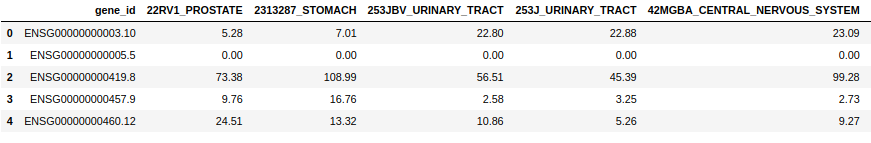
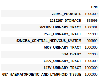
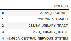

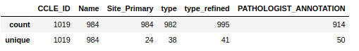
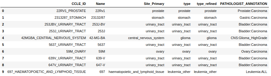
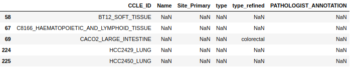

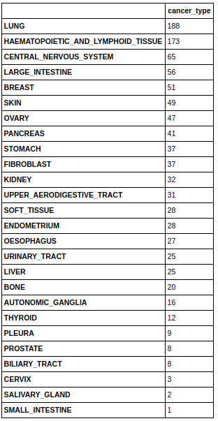
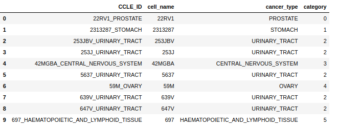
- 投稿日:2019-05-27T22:08:11+09:00
【Python】コラ用に遊戯王カード名の組み合わせを自動検索するためのツールを作成しました
概要
いつ頃からか、次のような画像コラがTwitterで流行りだしました。
— りめん⎷aおかもと (@wixossccc) May 26, 2019見ての通り遊戯王のカードを貼り合わせて任意の文字列を生成しています。
というわけで、どのカードを貼り合わせればいいかを自動生成するコードを考えてみました。データ収集方法
まず、遊戯王のカード名一覧のデータセットを見つけてくる必要があります。
しかし、遊戯王カードWikiや公式データベースなどを見る限り、「カードパックごとの一覧」はあっても「全カード一覧」はなかなか見つかりません(全カードの枚数から考えると当然ではあるが)。
そのため、頑張ってコピペするか、スクレイピングするコードを書くなどして対処しましょう。幸い私の場合、デュエルリンクスのカード名一覧をなんとかして入手できました。(著作権が怖いのでカード名リストは公開しません)自動生成する方法
Twitterを見る限り、「カード名の1文字だけ使用する」といったことも可能なようです。
そのため、自由度は極めて高く、事実上任意の文字列を作り出せると言っても過言ではないでしょう。
ただ、さすがに「全部1文字だけで組む」とかは見た目的につまらなくなりそうなので、なるべく長い部分文字列を利用するコードにしたいです。
そこで思いついたのが、N-gramを利用する方法です。まずこのように、部分文字列のデータをハッシュで蓄えておきます。# word_hash……部分文字列一覧。word_hash[部分文字列の長さ][部分文字列]={対象となるカードの番号一覧} word_hash: Dict[int, Dict[str, Set[int]]] = {} for name_index, name in enumerate(name_list): name_len = len(name) for begin_index in range(0, name_len): for end_index in range(begin_index + 1, name_len + 1): # begin_indexからend_indexまでの範囲で単語(name)を切り取ったのがslice_word slice_len = end_index - begin_index slice_word = name[begin_index:end_index] # ハッシュ(word_hash)に部分文字列(slice_word)を登録する if slice_len not in word_hash: word_hash[slice_len] = {} if slice_word not in word_hash[slice_len]: word_hash[slice_len][slice_word] = set() word_hash[slice_len][slice_word].add(name_index) # 何文字までの部分文字列が取れたかを算出する max_len = max(word_hash.keys()) min_len = min(word_hash.keys()) print(f'部分長:{min_len}-{max_len}')次に、対象文字列を先頭から見ていって、なるべく長い文字列がヒットするように検索します。
先ほど書いたように、「部分文字列は1文字だけでもOK」というゆるいルールですので、貪欲法でパパっと当てはめてしまいましょう。
(以下のコードでは実装をサボったので、MIN_WORD_LENが大きすぎるなどして探索に失敗すると無限ループになります)MAX_COUNT = 5 # 部分文字列に対する候補カード名を表示する最大件数 MIN_WORD_LEN = 1 # 部分文字列の最小長さ query_text = 'ホワイト・シチューをライスニカケる者を抹殺するエルフの剣士' # 合成対象の文字列 query_text_len = len(query_text) p = 0 while p < query_text_len: for q in range(max_len, min_len - 1, -1): # pからqまでの範囲で単語(query_text)を切り取ったのがsliced_query_text sliced_query_text = query_text[p:p+q] sliced_query_text_len = len(sliced_query_text) # 枝刈り if sliced_query_text_len < MIN_WORD_LEN: continue if sliced_query_text_len not in word_hash: continue if sliced_query_text not in word_hash[sliced_query_text_len]: continue # ヒットしたので候補カード名一覧をMAX_COUNT件まで表示 print(f'【{sliced_query_text}】:') count = 0 for name_index in word_hash[sliced_query_text_len][sliced_query_text]: print(f' {name_list[name_index]}') count += 1 if count >= MAX_COUNT: break p += sliced_query_text_len探索例
まずは冒頭の文字列から。探索結果が次のように表示されますので、
【ホワイト・】:
 ホワイト・ドルフィン
 ホワイト・ホーンズ・ドラゴン
【シ】:
 闇の住人シャドウキラー
 キャトルミューティレーション
 魔轟神獣ガナシア
 スカル・ビショップ
 チューンド・マジシャン
【チュー】:
 チューナーズ・ハイ
 チューン・ウォリアー
 パワード・チューナー
 ガーディアン・スタチュー
 レベル・リチューナー
【を】:
 不幸を告げる黒猫
 屍を貪る竜
 弓を引くマーメイド
 裁きを下す女帝
 7つの武器を持つハンター
【ライス】:
 ガーディアン・トライス
 閃光の双剣―トライス
【ニカ】:
 フレムベルグルニカ
 ドリル・バーニカル
 ボタニカル・ライオ
【ケ】:
 デビル・クラーケン
 ロケット・ジャンパー
 剣闘獣トラケス
 ケルドウ
 モルティング・エスケープ
【る者】:
 黒羽を狩る者
 命を食する者
 炎を支配する者
 炎を操る者
 魂を狩る者
【を】:
 不幸を告げる黒猫
 屍を貪る竜
 弓を引くマーメイド
 裁きを下す女帝
 7つの武器を持つハンター
【抹殺】:
 無情の抹殺
 抹殺の使徒
 戦士抹殺
【す】:
 団結するレジスタンス
 盲信するゴブリン
 暴走する魔力
 鏡鳴する武神
 裁きを下す女帝
【るエルフの剣士】:
 翻弄するエルフの剣士
ここから好きな文字列を選んでコラ画像を作ればいいです。例えば、
ホワイト・シチューをライスニカケる者を抹殺するエルフの剣士

[ホワイト・]ホーンズ・ドラゴン
  闇の住人[シ]ャドウキラー
       [チュー]ン・ウォリアー
          屍[を]貪る竜
      閃光の双剣―ト[ライス]
         フレムベルグル[ニカ]
           デビル・クラー[ケ]ン
                 魂を狩[る者]
                 7つの武器[を]持つハンター
                        [抹殺]の使徒
                        鏡鳴[す]る武神
                         翻弄す[るエルフの剣士]
といったふうに作成できます。他にもいろいろ作ってみましょう。
精神を刻む者ジェイス
=[精神]統一
 翼[を]織りなす者
 破邪の[刻]印
 龍脈に棲[む者]
 [ジ]ュラック・メテオ
 バード・フ[ェイス]

ミミミンミミミンウーサミン
=暗黒の[ミミ]ックLV1
 [ミ]イラの呼び声
 サモ[ン]オーバー
 暗黒の[ミミ]ックLV3
 リ[ミ]ッター・ブレイク
 ドラゴ[ンウ]ィッチ-ドラゴンの守護者-
 ラヴァルバ[ー]ナー
 [サ]イコ・デビル
 アロマージジャス[ミン]

メタルギアソリッドピースウォーカー
=[メタル]デビルゾア
 フェニックス・[ギア]・フリード
 E・HERO[ソリッド]マン
 森羅の実張り [ピース]
 [ウォー]ター・ドラゴン-クラスター
 サモンブレー[カー]
注意
- 言うまでもありませんが、ミリシタやシャニマスなどのカード名でも同様にコラ画像の種に使えます
- 暇な人は画像コラを作成する部分も自動作成してみると楽しいのではないでしょうか
- 投稿日:2019-05-27T21:40:07+09:00
GeoPandasがうまく実行できないときの対処法
GeoPandasのインストールが環境によって、うまくいかないという報告をよく受けるため、基本的なインストールで気をつけることを共有します。
インストール環境
virtualenvなどを用いて、まっさらな環境がおすすめ。別のパッケージで古いバージョンのパスを通していると2次災害が起きることがよくあるため。
インストール手順
GeoPandas=0.5.0(2019年5月時点で最新)の場合には、Githubの本家から直接インストールすることをおすすめします。PyPIに登録されているversionはoveralayの関数の修正が反映されていないようですが、github上では修正後版がmasterブランチにマージされているようです。
pip install pandas fiona shapely pyproj rtree descartes
pip install git+git://github.com/geopandas/geopandas.git
手っ取り早く使いたいときは...
GoogleDriveにパスを通すことが億劫でさえなければ、GoogleColaboratryを使うと簡単です。参考までにコード を共有します。
GeoPandasは使い勝手が不安定であることがもったいないです。Pandasとの互換性があり、とても便利ですので、普及を応援したいです。
- 投稿日:2019-05-27T20:57:59+09:00
PythonistaでGPS
はじめに
PythonistaでGPSが使えるらしいので試してみた。
実装
import location

location.start_updates() # GPSデータ更新を開始
gps_data=location.get_location() # GPSデータを取得する
location.stop_updates()# GPSデータ更新を終了

print(gps_data['latitude'])
print(gps_data['longitude'])
結果
かなり簡単にGPS情報を取得できた。
しかし、このままでは緯度、経度の生データなのでどこなのかはわからない。
住所変換ライブラリもあるらしいが、Pythonistaで使えるのだろうか?
- 投稿日:2019-05-27T19:18:03+09:00
PySnooper の文字列を取得
こんにちは、古内です。
今回は少し前にバズった PySnooper で標準出力ではなく、Python としての文字列として取得する方法をご紹介します。はじめに
以下が、経緯です。
また、公式ドキュメントが整っておらず、文字列を取得するやり方について見つからなかったので記事にしました。
コード自体はかなり適当に作られています。
本番環境で恒久的に運用することはしないでください。この記事では、以下のバージョンでのご紹介になります。
- Python: 3.7.2
- PySnooper: 0.0.39
読者の想定
- Python 構文が分かる人
- 手っ取り早く PySnooper の文字列を Slack 等に送りつけたい人
- New Relic 等がどうしても使えない環境でボトルネックをチェックしたい人
ソースコード
正直、記事にするか悩むレベルで簡単です。( ドキュメントなかったのでとりあえず記事にしましたが… )
https://github.com/furuuchitakahiro/get-PySnooper-string
https://github.com/furuuchitakahiro/get-PySnooper-string/blob/master/get_pysnooper_string.py#L13-L19
class MyWritableStream(pysnooper.utils.WritableStream):
    def __init__(self, *args, **kwargs):
        super().__init__(*args, **kwargs)
        self.dump_message = ''

    def write(self, s: str) -> None:
        self.dump_message += s
はい、ほぼこれだけです。
あとは使うだけ。https://github.com/furuuchitakahiro/get-PySnooper-string/blob/master/get_pysnooper_string.py#L5-L10
ws = MyWritableStream()
with pysnooper.snoop(output=ws):
    num1 = 1
    num2 = 2
    result = num1 + num2
print(ws.dump_message)  # ws.dump_message で文字列として取得できる
あなたのデバッグしたいコードを
with pysnooper.snoop(output=ws):の中に突っ込んでください。
例ではnum1 = 1からresult = num1 + num2部分です。
そして、最後にprint(ws.dump_message)部分を Slack なりメールなり、ログファイルなりにすればいいと思います。解説のしようがないレベルであれなので必要なことだけ列挙しておきます。
- pysnooper.utils.WritableStream を継承したクラスを作って write メソッドオーバーライドする
- with 構文で snoop する際に引数に予め初期化しておいた WritableStream インスタンスを渡す
以上です。
注意としてはデコレータでの使用は難しいって感じですかね。
理由としては WritableStream の初期化が問題です。
( デコレーターで試してませんが多分だめだと思います )あとがき
なんだかすごく内容の薄い記事になってしまいました。
そのうち PySnooper もどんどん整備されていけばこういった記事がなくても良くなると思います。
ですが、WritableStream について触れている文献も探すの面倒だったりしたのでやっちゃいました。
こうした方がいいよとか、間違いとかあればぜひご指摘お願いします。
ありがとうございました!
- 投稿日:2019-05-27T18:46:58+09:00
numpyのsumでaxisの適応順番で混乱したので備忘録
よくnumpy.sumのaxisで迷うのでその備忘録。
[[[1,2,3,4,5,6],
[2,3,4,5,6,7],
[3,4,5,6,7,8]],
[[1,2,3,4,5,6],
[2,3,4,5,6,7],
[3,4,5,6,7,8]]]とかなっているとaxisが何が何だか解らなくなるので簡単な判別法
。
一番外の[]がaxis=0で内側の[]に入るごとにaxisの値が一つずつ増えていく。例
C=[[[1,2,3,4,5,6],
[2,3,4,5,6,7],
[3,4,5,6,7,8]],
[[1,2,3,4,5,6],
[2,3,4,5,6,7],
[3,4,5,6,7,8]]]np.sum(C,axis=0)だと一番外のカッコ内レベルで計算されるので
array([[ 2, 4, 6, 8, 10, 12],
[ 4, 6, 8, 10, 12, 14],
[ 6, 8, 10, 12, 14, 16]])np.sum(C,axis=2)
外側から3番目のカッコ内を足すので
array([[21, 27, 33],
[21, 27, 33]])になる
- 投稿日:2019-05-27T17:51:42+09:00
Revit Api pyrevitでEnumを使う
sample.pyfrom rpw import DB from rpw.utils.dotnet import Enum for bip in Enum.GetValues(DB.BuiltInParameter): print bip for bip in Enum.GetNames(DB.BuiltInParameter): print bip print type(bip) for pt in Enum.GetValues(DB.ParameterType): print pt print type(pt)BuiltInParameterをrpwを使ってPythonで書くときにEnumをどこからインポートしたら良いか詰まりました。
Enum.GetValues()では'BuiltInParameter'、Enum.GetNames()だと'str'を返します。参考にしたリンクはこちら。
https://thebuildingcoder.typepad.com/blog/2011/08/built-in-parameter-name-and-labelutils.html
- 投稿日:2019-05-27T17:11:45+09:00
茶コーダーへの道 #3
プログラミング初心者が茶コーダーを目指す感動サクセスストーリー(?)です.目標は7月いっぱいまでに茶色になることです.温かい目で見てください.よろしくお願いします.この「茶コーダーへの道」では,Atcoderの過去問および競技プログラミングの問題の種類や解き方等々のついて個人的にまとめていきます.すごい人はアドバイスをいただければ幸いです.
諸事情により#3からスタート.
Atcoder Beginner Contest 127
先日のAtcoder Beginner Contest 127ですが,僕はA問題,B問題の2問の正解でした.
どうしてもC問題が解けず・・・残念・・・まずは,A問題.これは5分44秒で解けました.
abc127_a.pya,b=map(int,input().split()) if a<=5: print(0) elif 6<=a and a<=12: print(b//2) else: print(b)一行で書いている人,何者・・・
Atcoderの解説を見たら,最初のifで5歳以下かどうか判断をしているので,2つ目のelifの段階で6歳以上は確定している.つまり,6<=aはいらないということです.なるほど・・・こういうのを論理的な考え方というのでしょうか.次に,B問題.
abc127_b.pyr,d,x=map(int,input().split()) for i in range(10): x=r*x-d print(x)A問題より簡単だった?
これは5分かかってないですね.
A,B問題が終わり,10分38秒経過です.残り約90分をC問題に費やしました・・・しかし解けず.
当面の目標は「C問題を解けるようになる」ということで良さそう.C問題の公式解説を見た.「区間の数を求める時には最も制約の厳しいところに注目する.」ことがコツ.言われるとそうだ・・・
最後の行の
ans=max(ans,0)もなかなか僕は思いつかなそう.
ということで解説はC++で書いてるので,僕はPythonで書いてみた.abc127_c.pyN,M=map(int,input().split()) l=[list(map(int,input().split())) for i in range(M)] maxL=1 minR=N for j in range(M): maxL=max(maxL,l[j][0]) minR=min(minR,l[j][1]) ans=minR-maxL+1 ans=max(ans,0) print(ans)AC!素直に嬉しい.
追記.
Twitterを見ると,C問題はこれはiris法(?)と言っている人が多かった.
iris法とは何ぞやと調べてみた.
- 投稿日:2019-05-27T16:35:40+09:00
Anacondaの仮想環境を使ってkerasを使おう
Kerasの環境をつくろう
pip install tensorflow
pip install tensorflow-gpu //GPUを使う場合
pip install keras
一応これでkerasを使うことができる。
しかし、これではkerasやtensorflowと干渉するモジュールを使うPythonを使う場合や異なるpythonのバージョンを使いたい場合など、いちいちパッケージの削除やインストールをし直す必要がる。
そこで、Pythonには仮想環境というものがある。
Python仮想環境とは?なぜ仮想環境を使うのか?
PythonのモジュールやパッケージをPythonのバージョンごとに分割させた環境。
「あるパッケージを使うには別のパッケージをインストールする必要がある」など、Pythonのパッケージには依存関係がある。また、Pythonのバージョンによっても対応してたり対応してなかったりする場合もある。
仮想環境を使わないと、Pythonで作られたソフトウェアなどによって同じシステムですでに作られた環境を破壊したりする必要も出てくる。
仮想環境の種類
Pythonの仮想環境にはいろいろある
- pyenv
- virtualenv
- venv
- anaconda
など
とりあえず、Python3系であればanacondaかvenvが一番使いやすいと思われる。今回はanacondaを使おう。
anacondaをインストールしよう。
anacondaは以下からダウンロードできる。
- https://www.anaconda.com/distribution/自分の環境に合わせてダウンロードするanacondaを選ぼう。
GUI環境がなくてウェブブラウザが使えない
wgetを使おう。
$ wget https://repo.anaconda.com/archive/Anaconda3-2019.03-Linux-x86_64.shなおこのコマンドはPython3.7、Linux 64bit版のインストーラーがダウンロードされる。
各自バージョンや環境に合わせてURLに適切なものを選ぼう。
インストール
Linuxの場合は以下のコマンドでインストールが開始される。
$ bash Anaconda3-2019.03-Linux-x86_64.shライセンス許諾などいろいろ聞かれるが、デフォルトの選択を選んでおけばだいたい問題はないと思う。
anacondaのコマンドたち
よく使うコマンドなので覚えておくといいかもしれない。
なお以下のコマンドはLinuxで使う場合である。Windowsとかだとちょっと違うかもしれない。
インストールされているパッケージを表示する
$ conda listパッケージをインストールする
$ conda install kerasこのコマンドはkerasがインストールされる。"keras"の部分をインストールしたいパッケージに変えれば、そのパッケージがインストールされる。
新しい仮想環境を構築する。
$ conda create -n hoge python=3.7このコマンドは"hoge"という名前の仮想環境をPython3.7で構築する。
仮想環境に入る
$ conda activate hogehogeという仮想環境に入る
仮想環境から出る
$ conda deactivate間違えてexitとか入力しないように注意しよう。
仮想環境の一覧を表示
$ conda env list仮想環境を削除
$ conda env remove -n hogehogeという仮想環境が削除される。
改めて、Kerasを使って機械学習をする仮想環境を作ろう。
仮想環境を作ってその中に入ろう
$ conda create -n keras_env python=3.7
$ conda activate keras_env
1行目でkeras_envという仮想環境を作り、2行目でkeras_envに入る。
まず、Tensorflowをインストールしよう。
$ conda install tensorflowGPUを使いたい人は
$ conda install tensorflow-gpuそして、kerasをインストール。
$ conda install keras動作確認的な
下のリンクにMNISTのサンプルコードがあるのでコピペして実行してみよう
https://qiita.com/samacoba/items/207f2650ee60fe1de25a
おわりに
jupyter notebookをいい感じに使えるようにしたい。
- 投稿日:2019-05-27T16:31:43+09:00
Optuna と Chainer で深層学習のハイパーパラメータ自動最適化
はじめに
Optuna は、オープンソースのハイパーパラメータ自動最適化ツールです。この記事では、Optuna と Chainer を用いて、実際に深層学習(ディープラーニング)のハイパーパラメータ最適化を行う方法を説明します。Optuna の examples にはさまざまなフレームワークでの例が載っていますが、ドキュメントとして説明はされていないようなので、私なりにアレンジを加えたものを紹介します。
内容としては:
- ハイパーパラメータとは何か?
- Optuna でシンプルな最適化
- Optuna + Chainer で深層学習のハイパーパラメータ最適化
のようになっています。
対象とする読者は以下です:
- Chainer などの深層学習フレームワークに慣れ親しんでいる方
- Optuna のチュートリアルは触ったものの、そこから深層学習のハイパーパラメータ自動最適化に活用する方法がわからない方
反対に、対象と しない 読者は以下です:
- Optuna のチュートリアル をまだやっていない方 → まずはそちらやることをオススメします。
- Optuna の examples を読んで理解できる方 → それらを超える内容はほぼありません。
- 機械学習の基礎的な概念・Python の基本的な文法を知らない方 → この記事では説明しないので、ほかで習得してから読んでください。
また、この記事で解説するコードの完全なものは GitHub のリポジトリ にあります。
ハイパーパラメータとは何か?
深層学習の場合、ハイパーパラメータとは例えば層の数や活性化関数の種類など、学習の過程で変化しないパラメータを指します。実際に学習を行うときはそれらを決めた上で、それぞれの層が持っている重みやバイアスなどのパラメータを最適化することで学習を行うわけですが、層の数や活性化関数の種類は学習の過程で最適化されるわけではなく、あらかじめ人間が手で与える必要がありました。したがって、学習の過程で最適化されるパラメータ(層が持っている重みやバイアス)と区別するために、層の数や活性化関数の種類のことを ハイパーパラメータ と呼びます。以下に、深層学習におけるパラメータの例とハイパーパラメータの例を示します。
深層学習におけるパラメータの例:
- 層の重み
- 層のバイアス
深層学習におけるハイパーパラメータの例:
- 層の数
- 活性化関数の種類(ReLU や Sigmoid など)
- 最適化方法の種類(Adam や SGD など)
- 最適化方法のパラメータ(学習率など)
深層学習では誤差逆伝播を用いて勾配(loss のパラメータによる微分)を計算しパラメータのアップデートを行います。対してハイパーパラメータでは層の数や活性化関数の種類など、それを変えるとモデルの性質がドラスティックに変わるため微分が簡単に行えなそうなものが多いです。そういった意味でも、これらのハイパーパラメータは学習時に最適化することが難しく、学習を始める前に決めうちにならざるを得ないという背景もあります。
ハイパーパラメータ最適化のプロセス
人手によるハイパーパラメータ更新の例を以下に示します。例ではふたつの学習を同時に走らせていますが、学習が終わるごとに人手によるチェックが入るため、ハイパーパラメータを試せる数に限りがあり、またスケールもしません。例えば 100 個 GPU を用意して 100 セットのハイパーパラメータで同時に学習させることを考えてください。それらの学習が終わった際に、次にみるべきハイパーパラメータを即座に判断できるでしょうか?
一方で、Optuna などのハイパーパラメータ自動最適化ツールを使った場合の例をいかに示します。人手が入る時間は限られているため、学習が効率的に回せていることが見て取れます。また、この方法であれば、 100 セットのハイパーパラメータで同時に学習させたとしても、学習回数はそれに応じてスケールしていきます。詳しくは後で述べますが、結果を評価する際も、スジのよいハイパーパラメータだけを見ればよいため、評価を行うコストも実はそこまで高くありません。
以上より、ハイパーパラメータ自動最適化ツールを使ったほうがより効率的に機械学習プロセスを回せそうであることがわかりました。当然、実際にはすべての点で自動最適化が勝っているわけではありません。ハイパーパラメータ自動最適化ツールとはいえ、どのハイパーパラメータを最適化するかをあらかじめ指定する必要があります(ハイパーパラメータ自動最適化ツールのハイパーパラメータ!)が、そういった制約から完全に自由である、人手による最適化が勝る可能性もゼロではないからです。
とはいえ、人手では試せる回数も限られたものになりますので、ハイパーパラメータ自動最適化ツールより性能がよいハイパーパラメータを見つけられたとしてもそれは「たまたま」かもしれません。実務上ではこういった「たまたま」に頼るよりは、試行回数をできるだけ増やしてなるべくうまくいく確率を統計的に増やしていくことが求められると思います。また、近年ではハイパーパラメータ自動最適化を含む領域として AutoML という対象が盛んに研究されており、こういった方向性は今後より一層強まっていくと予想できます。
Optuna でシンプルな最適化
ではいよいよ Optuna で最適化を行っていきましょう。いきなり深層学習の最適化を行ってもわかりにくいので、まずはシンプルな例からいきましょう。
問題として、サインウェーブのフィッティングを考えます。範囲 $[0, 2 \pi]$ をとる $x$ に対して、
y = \sin xである $y$ を予測するモデルを、まずは多項式で立てます。
この際のハイパーパラメータとしては、多項式の次数を選びます。次数が 2 だったら 2 次関数で $\sin$ をフィッティングするということですね。
全体像
まずはコードの
main関数を示します。それぞれの関数やメソッドの中身はまだ説明していませんので、ここでは大まかなながれをつかんでいただければ十分です。流れとしては:
- データを作る
- ハイパーパラメータ最適化(
study)のための設定をする- 実際に最適化計算を行う
- もっともよかった結果を可視化する
といった流れとなっています。
from pathlib import Path

import optuna


STUDY_NAME = 'poly'
N_TRIALS = 10

MODEL_DIRECTORY = Path('models/poly')


def main():
    # Generate dataset
    prepare_dataset()

    # Prepare study
    if not MODEL_DIRECTORY.exists():
        MODEL_DIRECTORY.mkdir(parents=True)
    study = optuna.create_study(
        study_name=STUDY_NAME, storage=f"sqlite:///{STUDY_NAME}.db",
        load_if_exists=True)

    # Optimize
    study.optimize(objective, n_trials=N_TRIALS)

    # Visualize the best result
    print('=== Best Trial ===')
    print(study.best_trial)
    evaluate_results(study.best_trial)


if __name__ == '__main__':
    main()
studyというのが今考えているタスクに対するハイパーパラメータ自動最適化の計算ワンセットを指していて、ハイパーパラメータをひとつセットして学習を 1 回行うことはtrialと呼ばれています。trialがたくさんあつまってひとつのstudyをつくっているイメージですね。データの作成
ではデータを作りましょう。 $x$ として $[0, 2 \pi]$ の範囲をとる一様乱数を作り、それに $\sin$ を作用させます。また、機械学習で使うデータでは
(サンプルサイズ, 特徴量次元)の 2 次元配列になっていることが多いので、今回は特徴量次元を 1 として、(DATA_SIZE, 1)次元の配列としてxとyを作ります。import numpy as np DATA_SIZE = 1000 DATASET_DIRECTORY = Path(f"./data/dataset_{DATA_SIZE}") def generate_data(size=1000): """Generate training data. Args: length: int The sample size of the data. Returns: x_train: numpy.ndarray The input data for training. y_train: numpy.ndarray The output data for training. x_valid: numpy.ndarray The input data for validation. y_valid: numpy.ndarray The output data for validation. """ x = np.random.rand(size, 1).astype(np.float32) * 2 * np.pi y = np.sin(x) n_train = int(size * 0.8) return x[:n_train], y[:n_train], x[n_train:], y[n_train:]最後のところでは、データを train dataset と validation dataset に 8:2 の割合で分割しています。最適化計算のたびにデータを作るとデータが計算に時間がかかるばかりかデータも変わってしまうので、データがまだ作られていなかったらデータを作って保存する関数も別途作っておきます。
def prepare_dataset():
    """Prepare dataset for optimization."""
    if not DATASET_DIRECTORY.exists():
        DATASET_DIRECTORY.mkdir(parents=True)
        x_train, y_train, x_valid, y_valid = generate_data(DATA_SIZE)
        np.save(DATASET_DIRECTORY / 'x_train.npy', x_train)
        np.save(DATASET_DIRECTORY / 'y_train.npy', y_train)
        np.save(DATASET_DIRECTORY / 'x_valid.npy', x_valid)
        np.save(DATASET_DIRECTORY / 'y_valid.npy', y_valid)
目的関数
次はいよいよ Optuna に直接関係する部分の実装です。Optuna では最小化したい目的関数(Objective function)を定義し、ハイパーパラメータを変化させながら目的関数の値を評価することで、ハイパーパラメータ自動最適化を行います。
import pickle

from sklearn.linear_model import Ridge
from sklearn.preprocessing import PolynomialFeatures
from sklearn.pipeline import make_pipeline


def objective(trial):
    """Objective function to make optimization for Optuna.

    Args:
        trial: optuna.trial.Trial
    Returns:
        loss: float
            Loss value for the trial
    """

    # Suggest hyperparameters
    polynomial_degree = trial.suggest_int('polynomial_degree', 1, 10)

    print('--')
    print(f"Trial: {trial.number}")
    print('Current hyperparameters:')
    print(f"    Polynomial degree: {polynomial_degree}")
    print('--')

    # Generate the model
    model = make_pipeline(PolynomialFeatures(polynomial_degree), Ridge())

    # Load dataset
    x_train = np.load(DATASET_DIRECTORY / 'x_train.npy')
    y_train = np.load(DATASET_DIRECTORY / 'y_train.npy')
    x_valid = np.load(DATASET_DIRECTORY / 'x_valid.npy')
    y_valid = np.load(DATASET_DIRECTORY / 'y_valid.npy')

    # Train
    model.fit(x_train, y_train)

    # Save model
    with open(MODEL_DIRECTORY / f"model_{trial.number}.pickle", 'wb') as f:
        pickle.dump(model, f)

    # Evaluate loss
    loss = np.mean((model.predict(x_valid) - y_valid)**2)
    return loss
ちょっと関数としては長いですが、やっていることはそんなに多くありません。順番に説明していきましょう。
まずは引数ですが、これは
optuna.trial.Trialクラスのオブジェクトです。Optuna の最適化プロセスでは、このTrialオブジェクトを作ってはobjective関数に渡して評価して……というのを繰り返します。つまりこの引数は Optuna によって自動で与えられるため、ユーザ自らこのオブジェクトを作ってobjective関数を呼ぶことはあまりないと思います。この中で特に重要なのが
    # Suggest hyperparameters
    polynomial_degree = trial.suggest_int('polynomial_degree', 1, 10)
の部分でしょう。ここでひとつの
trialを行うためのハイパーパラメータを 1 セット(ここではpolynomial_degreeのみ)を生成しています。polynomial_degree(多項式の次数)は整数値をとるため、suggest_intメソッドを使ってハイパーパラメータを生成しています。引数の'polynomial_degree'はパラメータの名前(結果の表示などで必要です)、そのあとの1と10はハイパーパラメータのとりうる最小値と最大値です。つまり、1 次関数 〜 10 次関数の間でフィッティングを試みようとしているということです。他の部分はデータを読み込んだり、
sklearnのmodelを作成してデータにフィッティングし保存したりしている部分です。最後に# Evaluate loss loss = np.mean((model.predict(x_valid) - y_valid)**2) return lossの部分ですが、validation dataset に対してモデルによる推定を行い、正解との平均二乗誤差(
loss)を計算してそれをreturnしています。Optuna での最適化に使う目的関数の返り値は、必ず最小化したい値でなければいけません。結果の可視化
結果の可視化の部分も軽く触れておきます。この関数は、引数として与えられた
trialに対応するモデルのデータを読み込んで、validation dataset に対する結果をプロットするものです。import matplotlib.pyplot as plt def evaluate_results(trial): """Evaluate the optimization results. Args: study: optuna.trial.Trial Returns: None """ # Load model trial_number = trial.number with open( MODEL_DIRECTORY / f"model_{trial_number}.pickle", 'rb') as f: model = pickle.load(f) # Load data x_valid = np.load(DATASET_DIRECTORY / 'x_valid.npy') y_valid = np.load(DATASET_DIRECTORY / 'y_valid.npy') # Plot plt.plot(x_valid, y_valid, '.', label='answer') plt.plot(x_valid, model.predict(x_valid), '.', label='prediction') plt.legend() plt.show()main 関数ふたたび
ここでふたたび
main関数の部分を示します。def main(): # Generate dataset prepare_dataset() # Prepare study if not MODEL_DIRECTORY.exists(): MODEL_DIRECTORY.mkdir(parents=True) study = optuna.create_study( study_name=STUDY_NAME, storage=f"sqlite:///{STUDY_NAME}.db", load_if_exists=True) # Optimize study.optimize(objective, n_trials=N_TRIALS) # Visualize the best result print('=== Best Trial ===') print(study.best_trial) evaluate_results(study.best_trial)Optuna を直接使っている部分は
study = optuna.create_study以下なので、そこを説明します。まず
studyの作成部分ですが、study = optuna.create_study( study_name=STUDY_NAME, storage=f"sqlite:///{STUDY_NAME}.db", load_if_exists=True)このようになっています。
storage=f"sqlite:///{STUDY_NAME}.cb"となっていますが、これは変数が展開されてstorage=f"sqlite:///poly.cb"となります。この部分でstudyのデータをどこに保存するかを指定しています。ここでは SQLite を使っているため、インストールしてデータベースサーバを立ち上げた上で実行する必要があります。また、load_if_exists=Trueとしているので、すでに DB が存在していた場合はそのデータを読み込んで、最適化を再開します。もし SQLite 関連でうまくいかない場合は、該当する場所を
    study = optuna.create_study(
        study_name=STUDY_NAME)
のように書き換えてください。データが保存されませんが、SQLite のインストールなどは不要になります。
実際にハイパーパラメータの自動最適化を実行している部分は
study.optimize(objective, n_trials=N_TRIALS)です。目的関数として上で定義した
objectiveを与えており、それに基づいてN_TRIALSに指定した回数だけtrialを行い、studyを終了します。実行
全体のコードは こちら にありますので、
git cloneなどでダウンロードした上で、ターミナル上で$ python3 poly.pyとすれば、
data/dataset_1000にデータセットが作成され、モデルのパラメータがmodels/polyに保存されながら以下のような結果がターミナルに表示されるはずです。[I 2019-05-27 04:41:29,531] A new study created with name: poly -- Trial: 0 Current hyperparameters: Polynomial degree: 8 -- [I 2019-05-27 04:41:29,654] Finished trial#0 resulted in value: 0.0005262039485387504. Current best value is 0.0005262039485387504 with parameters: {'polynomial_degree': 8}. -- Trial: 1 Current hyperparameters: Polynomial degree: 2 -- [I 2019-05-27 04:41:29,754] Finished trial#1 resulted in value: 0.19891643524169922. Current best value is 0.0005262039485387504 with parameters: {'polynomial_degree': 8}. ... [I 2019-05-27 04:41:30,626] Finished trial#9 resulted in value: 0.004659125581383705. Current best value is 5.815048280055635e-05 with parameters: {'polynomial_degree': 5}. === Best Trial === FrozenTrial(number=2, state=<TrialState.COMPLETE: 1>, value=5.815048280055635e-05, datetime_start=datetime.datetime(2019, 5, 27, 4, 41, 29, 755017), datetime_complete=datetime.datetime(2019, 5, 27, 4, 41, 29, 843021), params={'polynomial_degree': 5}, distributions={'polynomial_degree': IntUniformDistribution(low=1, high=10)}, user_attrs={}, system_attrs={'_number': 2}, intermediate_values={}, params_in_internal_repr={'polynomial_degree': 5.0}, trial_id=3)最適化が終わったら、試した中でもっともスコアがよかった(
best_trial)ときのハイパーパラメータが表示されます。試されたハイパーパラメータとその結果はすべてデータベースに保存されているため、スコアの高い順に n 個データをとってくるなども簡単にでき、結果として人手によるチェックのコストを下げてくれています。私が実行したところによると、'polynomial_degree': 5のときに validation dataset に対するlossが5.815048280055635e-05で最小になったようです。また、それを用いた結果の可視化として下のようなグラフも表示されるはずです。
Optuna + Chainer で深層学習のハイパーパラメータ最適化
では Chainer で多層パーセプトロン(MLP)を作って、そのハイパーパラメータを Optuna で自動最適化してみましょう。タスクは先ほどと同様、$\sin$ のフィッティングとします。また、ハイパーパラメータとしては:
- 層の数
- 層を構成するユニットの個数
- 活性化関数
を選びました。
全体像
全体像自体もあまり変わりませんが、
main関数まわりをまず示します。import optuna STUDY_NAME = 'mlp' N_TRIALS = 100 PRUNER_INTERVAL = 100 def main(): # Generate dataset prepare_dataset() # Prepare study study = optuna.create_study( study_name=STUDY_NAME, storage=f"sqlite:///{STUDY_NAME}.db", load_if_exists=True, pruner=optuna.pruners.MedianPruner()) # Optimize study.optimize(objective, n_trials=N_TRIALS) # Visualize the best result print('=== Best Trial ===') print(study.best_trial) evaluate_results(study.best_trial) if __name__ == '__main__': main()ここで重要な変更はひとつだけで、
    study = optuna.create_study(
        study_name=STUDY_NAME, storage=f"sqlite:///{STUDY_NAME}.db",
        load_if_exists=True, pruner=optuna.pruners.MedianPruner())
のところです。新しい引数として
pruner=optuna.pruners.MedianPruner()を与えていますが、これは pruning (枝刈り)と呼ばれる、途中で明らかにダメそうな学習を早めに打ち切る機能です。人手でハイパーパラメータチューニングをするときも、10 epoch くらい走らせてみてダメそうだったら学習を止めて別のハイパーパラメータを試しますよね。それを機械がやってくれるということです。ただし、 pruning を行うには学習器自体にも設定が必要で、それは後述します。目的関数
データ生成の部分はまったく同じなので、目的関数から見ていきましょう。
from pathlib import Path

import chainer as ch
import optuna

PRUNER_INTERVAL = 100

EPOCH = 1000
DATA_SIZE = 5000
BATCH_SIZE = 100
GPU_ID = -1  # Set value >= 0 to use GPU (-1: CPU mode)

DATASET_DIRECTORY = Path(f"./data/dataset_{DATA_SIZE}")
MODEL_DIRECTORY = Path('models/mlp')


def objective(trial):
    """Objective function to make optimization for Optuna.

    Args:
        trial: optuna.trial.Trial
    Returns:
        loss: float
            Loss value for the trial
    """

    # Generate model
    classifier = generate_model(trial)

    # Create dataset
    x_train = np.load(DATASET_DIRECTORY / 'x_train.npy')
    y_train = np.load(DATASET_DIRECTORY / 'y_train.npy')
    x_valid = np.load(DATASET_DIRECTORY / 'x_valid.npy')
    y_valid = np.load(DATASET_DIRECTORY / 'y_valid.npy')

    # Prepare training
    train_iter = ch.iterators.SerialIterator(
        ch.datasets.TupleDataset(x_train, y_train),
        batch_size=BATCH_SIZE, shuffle=True)
    valid_iter = ch.iterators.SerialIterator(
        ch.datasets.TupleDataset(x_valid, y_valid),
        batch_size=BATCH_SIZE, shuffle=False, repeat=False)

    optimizer = ch.optimizers.Adam()
    optimizer.setup(classifier)
    updater = ch.training.StandardUpdater(train_iter, optimizer, device=GPU_ID)
    stop_trigger = ch.training.triggers.EarlyStoppingTrigger(
        monitor='validation/main/loss', check_trigger=(100, 'epoch'),
        max_trigger=(EPOCH, 'epoch'))

    trainer = ch.training.Trainer(
        updater, stop_trigger,
        out=MODEL_DIRECTORY/f"model_{trial.number}")

    log_report_extension = ch.training.extensions.LogReport(
        trigger=(100, 'epoch'), log_name=None)
    trainer.extend(log_report_extension)
    trainer.extend(ch.training.extensions.PrintReport(
        ['epoch', 'main/loss', 'validation/main/loss']))
    trainer.extend(ch.training.extensions.snapshot(
        filename='snapshot_epoch_{.updater.epoch}'))
    trainer.extend(ch.training.extensions.Evaluator(valid_iter, classifier))
    trainer.extend(ch.training.extensions.ProgressBar())
    trainer.extend(
        optuna.integration.ChainerPruningExtension(
            trial, 'validation/main/loss', (PRUNER_INTERVAL, 'epoch')))

    # Train
    trainer.run()

    loss = log_report_extension.log[-1]['validation/main/loss']
    return loss
処理は長くなっていますが、やっていることは多項式のときとそう変わりません。Chainer に慣れ親しんでいる方なら見慣れた処理が多いと思います(Updater や Trainer を使わずに Chainer をやっている方は、もったいないのでこのタイミングでそれらの使い方をおさえておきましょう)。ただ唯一
    trainer.extend(
        optuna.integration.ChainerPruningExtension(
            trial, 'validation/main/loss', (PRUNER_INTERVAL, 'epoch')))
のところは Optuna に由来する部分で、これが例の pruning のための設定その 2 です。いま
PRUNER_INTERVAL = 100としているので、 100 epoch おきに学習をとめるかどうか判断するという設定になっています。別途stop_triggerとして early stopping の設定もしていますので、
- 望みのなさそうなハイパーパラメータでの学習は早めに止める(pruning)
- 望みがありそうなハイパーパラメータでの学習でも、学習が停滞したら止める(early stopping)
の 2 重の構えになっています。したがって、最大のエポック数
EPOCH = 5000としていますが、私がためした限りでは 5000 epoch フルに学習が走った trial はありませんでした。適切なタイミングで学習を(自動的に)止めるのも、より多くのハイパーパラメータを試すための重要なファクターになっています。モデルの生成
上の目的関数のところで、モデルの生成部分は
    # Generate model
    classifier = generate_model(trial)
と、別の関数に置き換えてあっさり終わってしまっていました。実はこの部分こそが Optuna で深層学習をやるための重要な部分です。ハイパーパラメータ自動最適化ツールで深層学習を行いたい場合、もっとも重要なことは
- モデル生成をできるだけ柔軟にできるようにする
ことです。ハイパーパラメータ自動最適化ツールではハイパーパラメータを何か選んできてそれをもとにモデルを作るわけですが、裏を返せばモデル生成をパラメトリックに行える必要があります。ではそれを気にしながらモデル生成部分のコードを見ていきましょう。
def generate_model(trial):
    """Generate MLP model.

    Args:
        trial: optuna.trial.Trial
    Returns:
        classifier: chainer.links.Classifier
    """
    # Suggest hyperparameters
    layer_number = trial.suggest_int('layer_number', 2, 5)
    activation_name = trial.suggest_categorical(
        'activation_name', ['relu', 'sigmoid'])
    unit_numbers = [
        trial.suggest_int(f"unit_number_layer{i}", 10, 100)
        for i in range(layer_number - 1)] + [1]
    dropout_ratio = trial.suggest_uniform('dropout_ratio', 0.0, 0.2)

    print('--')
    print(f"Trial: {trial.number}")
    print('Current hyperparameters:')
    print(f"    The number of layers: {layer_number}")
    print(f"    Activation function: {activation_name}")
    print(f"    The number of units for each layer: {unit_numbers}")
    print(f"    The ratio for dropout: {dropout_ratio}")
    print('--')

    # Generate the model
    model = MLP(
        unit_numbers, activation_name=activation_name,
        dropout_ratio=dropout_ratio)
    classifier = ch.links.Classifier(
        model, lossfun=ch.functions.mean_squared_error)
    classifier.compute_accuracy = False
    return classifier
モデル生成部分はこのようになっており、前半部分は
trial.suggest_***でそれぞれに合った型のハイパーパラメータを生成しています。unit_numbers(各層を構成するユニットの個数)はintの配列ですが、layer_number(層の数)によって配列の長さ(=ハイパーパラメータの個数)が動的に変わります。こういった、ハイパーパラメータの数が動的に変化するような問題に対しても最適化を行える柔軟性が Optuna の長所のひとつだと思います1。また、今回は MLP の出力(y)の特徴量次元は 1 なので、unit_numbersの末尾に 1 を付け足しています。このようにして作成されたハイパーパラメータは、たとえばCurrent hyperparameters: The number of layers: 4 Activation function: sigmoid The number of units for each layer: [36, 99, 87, 1] The ratio for dropout: 0.6906857740018953のようになっています。
ハイパーパラメータが無事生成できたところで、モデルの具体的な生成の実装に移っていきます。モデルの実装は以下のようになっています。
class MLP(ch.ChainList):
    """Multi Layer Perceptron."""

    def __init__(
            self, unit_numbers, activation_name, dropout_ratio):
        """Initialize MLP object.

        Args:
            unit_numbers: list of int
                List of the number of units for each layer.
            activation_name: str
                The name of the activation function applied to layers except
                for the last one (The activation of the last layer is always
                identity).
            dropout_ratio: float
                The ratio of dropout. Dropout is applied to all layers.
        Returns:
            None
        """
        super().__init__(*[
            ch.links.Linear(unit_number)
            for unit_number in unit_numbers])
        self.activations = [
            self._create_activation_function(activation_name)
            for _ in self[:-1]] \
            + [ch.functions.identity]  # The last one is identity
        self.dropout_ratio = dropout_ratio

    def _create_activation_function(self, activation_name):
        """Create activation function.

        Args:
            activation_name: str
                The name of the activation function.
        Returns:
            activation_function: chainer.FunctionNode
                Chainer FunctionNode object corresponding to the input name.
        """
        if activation_name == 'relu':
            return ch.functions.relu
        elif activation_name == 'sigmoid':
            return ch.functions.sigmoid
        elif activation_name == 'identity':
            return ch.functions.identity
        else:
            raise ValueError(f"Unknown function name {activation_name}")

    def __call__(self, x):
        """Execute the NN's forward computation.

        Args:
            x: numpy.ndarray or cupy.ndarray
                Input of the NN.
        Returns:
            y: numpy.ndarray or cupy.ndarray
                Output of the NN.
        """
        h = x
        for i, link in enumerate(self):
            h = link(h)
            if i + 1 != len(self):
                h = ch.functions.dropout(h, ratio=self.dropout_ratio)
            h = self.activations[i](h)
        return h
ChainListクラスを継承してMLPクラスを定義しました。ChainListは層の数がわかっていなくても定義が書けるので、このような場合には重宝します。重要なメソッドをひとつひとつ見ていきます。まずはオブジェクトの初期化部分ですが、def __init__( self, unit_numbers, activation_name, dropout_ratio): """Initialize MLP object. Args: unit_numbers: list of int List of the number of units for each layer. activation_name: str The name of the activation function applied to layers except for the last one (The activation of the last layer is always identity). dropout_ratio: float The ratio of dropout. Dropout is applied to all layers. Returns: None """ super().__init__(*[ ch.links.Linear(unit_number) for unit_number in unit_numbers]) self.activations = [ self._create_activation_function(activation_name) for _ in self[:-1]] \ + [ch.functions.identity] # The last one is identity self.dropout_ratio = dropout_ratioのようになっています。
unit_numbersの長さの分だけchainer.links.Linearオブジェクト(重みとバイアス)が生成されていることがわかると思います。また、self.activationsでは各層の活性化関数を定義しているのですが、出力層のみchainer.functions.identity(恒等写像=何もしない関数)、ほかはハイパーパラメータとして与えられたactivation_nameをとるようにしています。ネットワークの foward 部分は、以下のようになっています。こちらでは層の数だけループを回して、線形変換とドロップアウト、活性化関数の適用を行っています。ただし、出力層にはドロップアウトを適用しないようにしています。
    def __call__(self, x):
        """Execute the NN's forward computation.

        Args:
            x: numpy.ndarray or cupy.ndarray
                Input of the NN.
        Returns:
            y: numpy.ndarray or cupy.ndarray
                Output of the NN.
        """
        h = x
        for i, link in enumerate(self):
            h = link(h)
            if i + 1 != len(self):
                h = ch.functions.dropout(h, ratio=self.dropout_ratio)
            h = self.activations[i](h)
        return h
結果の可視化
残るは結果の可視化の部分です。こちらも多項式のときと同様、指定された
trialに対応するモデルをロードして推測させ、答えと比較しています。def evaluate_results(trial): """Evaluate the optimization results. Args: study: optuna.trial.Trial Returns: None """ # Load model trial_number = trial.number unit_numbers = [] for i in range(100): param_key = f"unit_number_layer{i}" if param_key not in trial.params: break unit_numbers.append(trial.params[param_key]) model = MLP( unit_numbers + [1], trial.params['activation_name'], trial.params['dropout_ratio']) snapshots = glob.glob(str(MODEL_DIRECTORY / f"model_{trial_number}" / '*')) latest_snapshot = max( snapshots, key=os.path.getctime) # The latest snapshot of the trial print(f"Loading: {latest_snapshot}") ch.serializers.load_npz( latest_snapshot, model, path='updater/model:main/predictor/') # Load data x_valid = np.load(DATASET_DIRECTORY / 'x_valid.npy') y_valid = np.load(DATASET_DIRECTORY / 'y_valid.npy') # Plot plt.plot(x_valid, y_valid, '.', label='answer') with ch.using_config('train', False): predict = model(x_valid).data plt.plot(x_valid, predict, '.', label='prediction') plt.legend() plt.show()まず予備知識として、
trial.paramsは例えば{'activation_name': 'sigmoid', 'dropout_ratio': 0.1948279849856978, 'layer_number': 5, 'unit_number_layer0': 77, 'unit_number_layer1': 56, 'unit_number_layer2': 51, 'unit_number_layer3': 80}のような辞書型のオブジェクトとしてその trial のハイパーパラメータを保持しています。したがって、これらのハイパーパラメータを使ってモデルを再構成し、(ハイパーでない)パラメータを読み込めばいいわけです。パラメータの読み込みでは、その trial のもっとも新しい snapshot を見つけてきてそれを読み込んでいます。ちょっとややこしいのが
unit_numbersを読み込んでいるところで、unit_numbersの長さが不定のため、ひとつひとつ読みながら配列に要素を追加していっています。このあたりが Optuna にがんばってほしいところで、配列などもハイパーパラメータとして扱えるようになればかなり取り回しがしやすくなると思います。実行
全体のコードは こちら にありますので、
git cloneなどでダウンロードした上で、ターミナル上で$ python3 mlp.pyとすれば、モデルのパラメータが
models/mlpに保存されながら以下のような結果がターミナルに表示されるはずです。[I 2019-05-27 15:26:18,496] Using an existing study with name 'mlp' instead of creating a new one. -- Trial: 0 Current hyperparameters: The number of layers: 3 Activation function: sigmoid The number of units for each layer: [83, 80, 1] The ratio for dropout: 0.043383365517199284 -- epoch main/loss validation/main/loss 100 0.131512 0.123286 200 0.0594965 0.0570084 300 0.0364821 0.0299548 400 0.0196009 0.00784213 500 0.014053 0.00332701 600 0.0111817 0.0023173 700 0.00912656 0.00166577 800 0.00797004 0.00153381 900 0.006777 0.0012653 1000 0.00608755 0.00110705 1100 0.00560331 0.00109022 1200 0.00517723 0.00108871 1300 0.00489841 0.00112543 1400 0.00468537 0.00100757 1500 0.00446898 0.000979245 1600 0.00428505 0.000921101 1700 0.00424085 0.000983566 1800 0.00405002 0.000959924 1900 0.00384459 0.000955113 [I 2019-05-27 15:28:03,244] Finished trial#0 resulted in value: 0.0009551127247686964. Current best value is 0.0009551127247686964 with parameters: {'activation_name': 'sigmoid', 'dropout_ratio': 0.043383365517199284, 'layer_number': 3, 'unit_number_layer0': 83, 'unit_number_layer1': 80}. -- Trial: 1 Current hyperparameters: The number of layers: 5 Activation function: relu The number of units for each layer: [53, 87, 75, 12, 1] The ratio for dropout: 0.10755231083048578 -- epoch main/loss validation/main/loss 100 0.249045 0.225993 200 0.0869799 0.0862519 ... === Best Trial === FrozenTrial(number=1, state=<TrialState.COMPLETE: 1>, value=0.00015463905489013997, datetime_start=datetime.datetime(2019, 5, 27, 7, 15, 22, 258062), datetime_complete=datetime.datetime(2019, 5, 27, 7, 16, 59, 707008), params={'activation_name': 'sigmoid', 'dropout_ratio': 0.0032366848483553535, 'layer_number': 3, 'unit_number_layer0': 41, 'unit_number_layer1': 18}, distributions={'activation_name': CategoricalDistribution(choices=('relu', 'sigmoid')), 'dropout_ratio': UniformDistribution(low=0.0, high=0.2), 'layer_number': IntUniformDistribution(low=2, high=5), 'unit_number_layer0': IntUniformDistribution(low=10, high=100), 'unit_number_layer1': IntUniformDistribution(low=10, high=100)}, user_attrs={}, system_attrs={'_number': 1}, intermediate_values={100: 0.0697100069373846, 200: 0.04887961223721504, 300: 0.036658125929534435, 400: 0.01331155956722796, 500: 0.001735480735078454, 600: 0.00048741648788563907, 700: 0.00028684467542916536, 800: 0.0001745481313264463, 900: 0.0001783440457074903, 1000: 0.00014417021156987175, 1100: 0.00017049246162059717, 1200: 0.00015490048099309206, 1300: 0.0001087129203369841, 1400: 0.00011426526543800719, 1500: 0.0001357111832476221, 1600: 0.00020704924827441573, 1700: 0.00016470269474666566}, params_in_internal_repr={'activation_name': 1.0, 'dropout_ratio': 0.0032366848483553535, 'layer_number': 3.0, 'unit_number_layer0': 41.0, 'unit_number_layer1': 18.0}, trial_id=2)途中で
--
Trial: 98
Current hyperparameters:
    The number of layers: 4
    Activation function: sigmoid
    The number of units for each layer: [22, 49, 60, 1]
    The ratio for dropout: 0.8962421296002223
--
epoch       main/loss   validation/main/loss
Exception in main training loop: Trial was pruned at epoch 50.]  5.00%
Traceback (most recent call last):............................]  0.00%
  File "/usr/local/var/pyenv/versions/3.7.3/lib/python3.7/site-packages/chainer/training/trainer.py", line 319, in runers/sec. Estimated time to finish: 0:01:00.705030.
    entry.extension(self)
  File "/usr/local/var/pyenv/versions/3.7.3/lib/python3.7/site-packages/optuna/integration/chainer.py", line 109, in __call__
    raise optuna.structs.TrialPruned(message)
Will finalize trainer extensions and updater before reraising the exception.
[I 2019-05-27 05:59:31,203] Setting status of trial#98 as TrialState.PRUNED. Trial was pruned at epoch 50.
のような出力が出ていたら、その trial は Pruning されているということで、Pruning が動いていることも確認できると思います。最適化が終わったら(20 〜 30 分ほどかかるかもしれませんので、ログを眺めつつこの記事を読み返してみるのもいいかもしれません)、下のようなグラフも表示されるはずです(タスクが単純すぎたので、多項式よりよくなっているわけではないのが世知辛いですが)。
おわりに
この記事では、簡単なデータを作成して、その回帰問題に対して Optuna によるハイパーパラメータ最適化を行う方法を解説しました。Optuna は機械学習タスクのハイパーパラメータ最適化だけでなく、さまざまなブラックボックス最適化にもつかえるようなジェネラルなフレームワークだと思います。これを使いこなすことによって最適化タスクが格段に便利になることは確かだと思いますので、ぜひ使いこなして業務を効率化していきましょう!
ただし、実用上はユニットの数を層によってばらつかせることはあまりなく、中間層のユニット数は同じにすることが多いかもしれません。ここでは、Optuna のキャパシティを見るためにもあえて層ごとにユニット数を変えています。 ↩
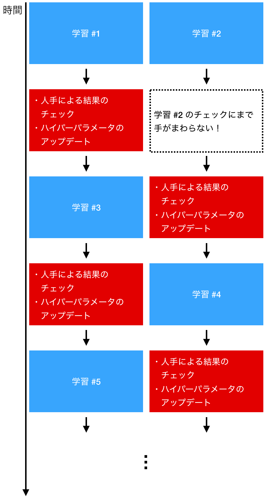
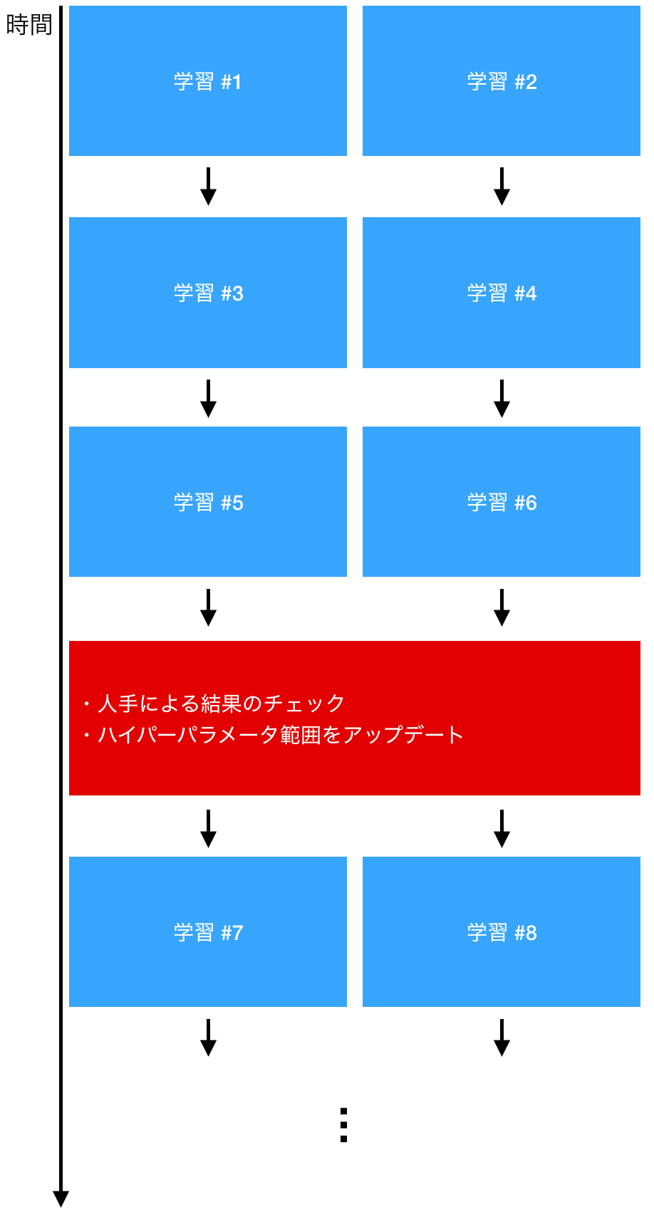
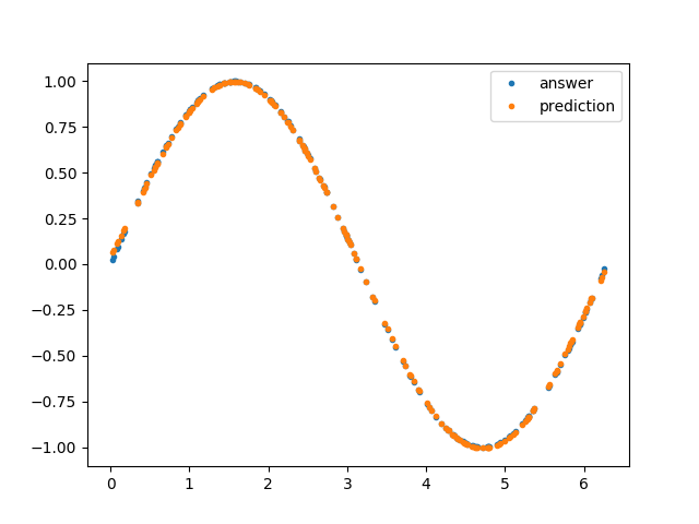
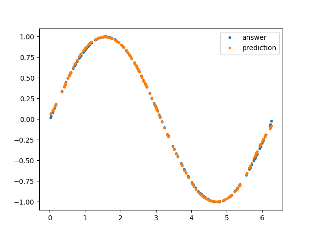
- 投稿日:2019-05-27T14:39:27+09:00
NumPyの使い方一覧
NumPyとは
NumPyはPythonの拡張モジュールで、ベクトルや行列などの演算などを行うことができます。
人工知能フレームワークの入力に使われていたりますので、人工知能を勉強する上で使い方を知っておくことは重要です。
あと、Atcoderでも使用できるため、NumPyで簡単に解ける問題もあるかもしれません。ここでは、NumPyでできることをまとめています。
NumPyのインストール
pipを使えば、以下のコマンドでNumPyを簡単にインストールすることが出来ます。
# pip install numpyNumPyのインポート
以下の「おまじない」でNumPyの使用が可能になります。省略名は「np」にすることが多いようです。
以降のコードは、この「おまじない」が実行済みであることを前提に記述します。import numpy as npNumPy配列の作成
array()にpythonのリスト型を渡すことで、NumPy配列を返してくれます。
一次元のリストを渡せばベクトル。二次元のリストなら行列。n次元のリストであればn階のテンソルとなります。ベクトル(1階のテンソル)
スカラー(数値)を縦、または横に並べたもの。
\vec{p} =
\left(
\begin{matrix}
p_1 \\
p_2 \\
\vdots \\
p_n
\end{matrix}
\right)

\qquad
or
\qquad

\vec{p} = (p_1, p_2, \cdots, p_n)
# ベクトル # P = [0 1 2 3 4 5] P = np.array([0, 1, 2, 3, 4, 5])行列(2階のテンソル)
ベクトルをストライプ状になるように並べたもの。縦を列、横を行と呼ぶ。
なので以下は、m行n列の行列となる。P = \left( \begin{matrix} p_{11} & p_{12} & \cdots & p_{1n} \\ p_{21} & p_{22} & \cdots & p_{2n} \\ \vdots & \vdots & \ddots & \vdots \\ p_{m1} & p_{m2} & \cdots & p_{mn} \\ \end{matrix} \right)# 行列 # P = [[1 2 3] # [4 5 6] # [7 8 9]] P = np.array([[1, 2, 3], [4, 5, 6], [7, 8, 9]])n階のテンソル
n-1階のテンソルを並べたもの。
# 3階のテンソル
P = np.array([[[0, 1, 2],
               [3, 4, 5],
               [6, 7, 8]],
              [[9, 8, 7],
               [6, 5, 4],
               [3, 2, 1]]])
全ての要素が「0.」のNumPy配列
zeros()で、全ての要素が「0.」のNumPy配列を作成できます。要素の型は浮動小数点数型となります。
# P = [0. 0. 0. 0. 0.]
P = np.zeros(5)

# 行列を作成したい場合は、タプルを引数にします
# P = [[0. 0.]
#      [0. 0.]]
P = np.zeros((2, 2))
未初期化のNumPy配列
empty()で、未初期化のNumPy配列を作成できます。要素の型は浮動小数点数型となります。
未初期化であるため、要素にははちゃめちゃな値が入っている場合がありますが、zeros()より高速のようです。
使い方はzeros()と同じです。# P = [0. 0. 0. 0. 0.] P = np.empty(5) # 行列を作成したい場合は、タプルを引数にします # P = [[0. 0.] # [0. 0.]] P = np.empty((2, 2))単位行列
単位行列とは、以下の様に「1」が斜めに並んだ正方行列で、「1」以外の要素は全て「0」です。
E = \left( \begin{matrix} 1 & 0 & \cdots & 0 \\ 0 & 1 & \cdots & 0 \\ \vdots & \vdots & \ddots & \vdots \\ 0 & 0 & \cdots & 1 \\ \end{matrix} \right)とある正方行列Aがある場合、単位行列Eと行列積をとっても値が変化しない特徴があります。
A =
\left(
\begin{matrix}
1 & 2 \\
3 & 4 \\
\end{matrix}
\right)

\qquad

E =
\left(
\begin{matrix}
1 & 0 \\
0 & 1 \\
\end{matrix}
\right)
AE = EA = \left( \begin{matrix} 1 & 2 \\ 3 & 4 \\ \end{matrix} \right)NumPyのeye()で、単位行列を作成できます。
# 引数は作成する単位行列の縦・横の大きさ # P = [[1. 0.] # [0. 1.]] P = np.eye(2)range()の様にNumPy配列を作成
Pythonのrange()は徐々に増加するlist型を返却してくれます。
NumPyのarange()を使えば、同じ様にNumPy配列を返却してくれます。# P = [0 1 2 3 4] P = np.arange(5) # P = [1 3 5 7 9] P = np.arange(1, 10, 2)NumPy配列の情報取得
NumPy配列にすると、配列の情報が簡単に取得できます。
NumPy配列のサイズ、NumPy配列の型
NumPy配列は、shapeでサイズ、dtypeで型を調べることができます。
# 行列
P = np.array([[1, 2, 3],
              [4, 5, 6],
              [7, 8, 9]])

# NumPy配列のサイズ (行のサイズ, 列のサイズ)で出力される
# (3, 3)
P.shape

# NumPy配列の型
# dtype('int64')
P.dtype
合計値、最大値、最小値
NumPy配列は、sum()により合計値、max()により最大値、min()により最小値を求めることができます。
# 行列
P = np.array([[1, 2, 3],
              [4, 5, 6],
              [7, 8, 9]])

# 合計値
# a = 45
a = np.sum(P)
a = P.sum()

# 最大値
# b = 9
b = np.max(P)
b = P.max()

# 最小値
# c = 1
c = np.min(P)
c = P.min()
平均値、分散、標準偏差
NumPy配列は、average()により平均、var()により分散、std()により標準偏差を求めることができます。
# 行列
P = np.array([[1, 2, 3],
              [4, 5, 6],
              [7, 8, 9]])

# 平均値
# a = 5.0 (45 / 9 = 5)
a = np.average(P)
a = P.mean()

# 分散
# b = 6.666666666666667
b = np.var(P)
b = P.var()

# 標準偏差
# c = 2.581988897471611
c = np.std(P)
c = P.std()
NumPy配列に「True」が含まれるか
NumPyのany()使用するとこで、NumPy配列に「True」が含まれるか判定できます。
この場合、以下の値は「False」であると判断されます。
- 論理型の「False」
- 数値型の「0」
- 浮動小数点型の「0.0」
# bools_1 = [False False True]
bools_1 = np.array([False, False, True])

# True
bools_1.any()

# bools_2 = [0 0.0 0]
bools_2 = np.array([0, 0.0, 0])

# False
bools_2.any()
NumPy配列が全て「True」であるか
NumPyのall()使用するとこで、NumPy配列の要素が全て「True」になっているか判定できます。
この場合、以下の値は「False」であると判断されます。
- 論理型の「False」
- 数値型の「0」
- 浮動小数点型の「0.0」
# bools_1 = [True True True]
bools_1 = np.array([True, True, True])

# True
bools_1.all()

# bools_2 = [True True False]
bools_2 = np.array([True, True, False])

# False
bools_2.all()
NumPy配列の操作
NumPy配列に対して行える操作について紹介します。
NumPy配列のハードコピー
NumPy配列は、copy()によりハードコピーを取得できます。
# P = [1 2 3]
P = np.array([1, 2, 3])

# P_copy = [1 2 3]
P_copy = P.copy()

# P      = [4 2 3]
# P_copy = [1 2 3]
P[0] = 4
NumPy配列のソート
NumPy配列はsort()により、ソートを行うことができます。
# P = [2 1 3]
P = np.array([2, 1, 3])

# 昇順にソート
# P_new = [1 2 3]
P_new = np.sort(P)

# NumPy配列のsort()メソッドを使用すると、NumPy配列自体が更新される
# P = [1 2 3]
P.sort()

# 降順にしたい場合は、[::-1]を付けると逆順となり降順となる
# P_reverse = [3 2 1]
P_reverse = P[::-1]
NumPy配列から重複を排除
NumPyのunique()使用すると、引数のNumPy配列から重複する要素が削除されたNumPy配列を取得できます。
countries = np.array(['France', 'Japan', 'USA', 'Russia', 'USA', 'Mexico', 'Japan'])

# 'USA'と'Japan'は重複しているので、1つなる
# countries_new = [France' 'Japan' 'Mexico' 'Russia' 'USA']
countries_new = np.unique(countries)
任意の値を配列が含むか確認
NumPyのin1d()使用すると、第一引数の配列の各要素が、それぞれ第二引数の配列に含まれているか判定することができます。
引数となる配列はNumPy配列だけでなく、Pythonのlist型でも動作するようです。
判定結果は真偽値のNumPy配列として返却されます。countries = np.array(['France', 'Japan', 'USA', 'Russia', 'USA', 'Mexico', 'Japan']) # 'Sweden'は含まれていないので False # ans = [True True False] ans = np.in1d(['France', 'USA', 'Sweden'], countries)条件を満たす要素だけ処理
NumPyのwhere()使用するとこで、条件を満たす要素に対して処理を実行できます。
# P = [[1 2],
#      [3 4]]
P = np.array([[1, 2], [3, 4]])

# 要素が3未満であれば「True」、そうでない場合は「False」を返却
# ans = [[True  True],
#        [False False]]
ans = np.where(P < 3, True, False)

# 要素が3未満であれば「3」、そうでない場合はそのままの値を返却
# ans_2 = [[3 3],
#          [3 4]]
ans_2 = np.where(P < 3, 3, P)
NumPy配列の形状変換
NumPy配列はreshape()により、形状変換後の新たなNumPy配列を取得できます。
# P = [0 1 2 3 4 5 6 7]
P = np.arange(8)

# 二次元以上の形状にする場合、引数はタプルで指定
# P2 = [[0, 1, 2, 3],
#       [4, 5, 6, 7]]
P2 = P.reshape((2,4))

# P3 = [[[0, 1],
#        [2, 3]],
#       [[4, 5],
#        [6, 7]]]
P3 = P.reshape((2,2,2))

# 一次元の形状にする場合、引数は整数型で指定
# P1 = [0 1 2 3 4 5 6 7]
P1 = P3.reshape(8)
ただし、NumPy配列の要素数が形状変換で指定したものと合わない場合はエラーになります。
# P = [0 1 2 3 4 5 6 7]
P = np.arange(8)

# ValueError: cannot reshape array of size 8 into shape (3,3)
P  = P.reshape(9)
P2 = P.reshape((3, 3))
行列の転置
行列を転置すると、行と列が入れ替わります。
A =
\left(
\begin{matrix}
a & b \\
c & d \\
e & f \\
\end{matrix}
\right)

\qquad

A^T =
\left(
\begin{matrix}
a & c & e \\
b & d & f \\
\end{matrix}
\right)
行列積を行う場合、基本的に前の行列の列数と、後ろの行列の行数が一致している必要があります。
しかし、一致していない行列でも、転置することで行列積が可能になる場合があります。NumPy配列はTまたは、transpose()で、転置後の新たなNumPy配列を取得できます。
# P = [[1 2]
#      [3 4]]
P = np.array([[1, 2],
              [3, 4]])

# PT = [[1 3]
#       [2 4]]
PT = P.T
PT = P.transpose()
行列の軸(axis)の入替え
NumPy配列はswapaxes()で、軸(axis)入替えが可能です。
軸(axis)入替え後の新たなNumPy配列を取得できます。# P = [[1 2] # [3 4]] P = np.array([[1, 2], [3, 4]]) # 引数に入替えを行う軸(axis)を指定 # 行列の場合、行が「axis = 1」、列が「axis = 0」となります # PT = [[1 3] # [2 4]] PT = P.swapaxes(1, 0)逆行列と行列式
以下のように、行列積を行うと単位行列になる互いの行列が存在する場合、それらの行列は逆行列の関係にあります。
この際、これらの行列は行と列の数が等しい正方行列である必要があります。A A^{-1} = A^{-1}A = Eまた、行列式が「0」となる行列は逆行列が存在しません。
行列Aの行列式|A|は、以下のように求められます。A = \left( \begin{matrix} a & b \\ c & d \\ \end{matrix} \right)|A| = ad - bc逆行列が存在する場合、以下の公式にから逆行列を求めることができます。
A^{-1} = \frac{1}{ad - bc} \ \left( \begin{matrix} d & -b \\ -c & a \\ \end{matrix} \right)NumPyではlinalg.det()で行列式を、linalg.inv()で逆行列を取得できます。
# A = [[1 2]
#      [3 4]]
A = np.array([[1, 2],
              [3, 4]])

# B = [[1 2]
#      [0 0]]
B = np.array([[1, 2],
              [0, 0]])

# 行列式:逆行列が存在
# a = -2.0
a = np.linalg.det(A)

# 行列式:逆行列が存在しない
# b = 0.0
b = np.linalg.det(B)

# A_1 = [[-2    1  ]
#        [ 1.5 -0.5]]
A_1 = np.linalg.inv(A)

# 行列式が「0」のため、エラーとなる
# LinAlgError: Singular matrix
B_1 = np.linalg.inv(B)
固有値と固有ベクトル
とある正方行列Aに対して、以下の関係を満たすスカラーλを行列Aの固有値、ベクトル$\vec{x}$を行列Aの固有ベクトルといいます。
A\vec{x} = λ\vec{x}NumPyではlinalg.eig()で固有値と固有ベクトルを取得できます。
# P = [[3 1],
#      [2 4]]
P = np.array([[3, 1], [2, 4]])

# 戻り値evは、2つのNumPy配列から構成される
ev = np.linalg.eig(P)

# ev[0]が固有値
# ev[0] = [2. 5.]
ev[0]

# ev[1]が固有ベクトル
# ev[1] = [[-0.70710678 -0.4472136 ],
#          [ 0.70710678 -0.89442719]]
ev[1]
NumPyの演算機能
平方根や行列積など、NumPyの演算機能を紹介します。
三角関数
三角関数はNumPyのsin()、cos()、tan()で、それぞれ求めることができます。
引数はラジアンで指定する必要があります。# a = 0.8414709848078965 a = np.sin(1) # b = 0.5403023058681398 b = np.cos(1) # c = 1.557407724654902 c = np.tan(1)NumPy配列を引数にした場合は、全ての要素に対して三角関数を求めます。
# P = [0 1]
P = np.array([0, 1])

# a = [0.        0.84147098]
a = np.sin(P)

# b = [1.        0.54030231]
b = np.cos(P)

# c = [0.        1.55740772]
c = np.tan(P)
平方根
NumPyのsqrt()で平方根を求めることができます。
# a = 2.0
a = np.sqrt(4)
NumPy配列を引数にした場合は、全ての要素に対して平方根を求めます。
# P = [[1 2]
#      [3 4]]
P = np.array([[1, 2],
              [3, 4]])

# P2 = [[1          1.41421356]
#       [1.73205081 2         ]]
P2 = np.sqrt(P)
自然対数の底「e」の累乗
NumPyのexp()で「e」の累乗を求めることができます。
# a = 2.718281828459045
a = np.sqrt(1)
NumPy配列を引数にした場合は、全ての要素に対して、「e」の累乗を求めます。
# P = [[1 2]
#      [3 4]]
P = np.array([[1, 2],
              [3, 4]])

# P2 = [[ 2.71828183  7.3890561 ]
#       [20.08553692 54.59815003]]
P2 = np.exp(P)
行列積
行列Aと行列Bの行列積は、以下の様に表せます。
また、行列積を計算するためには、前の行列の列数と、後ろの行列の行数が一致していなければいけません。A = \left( \begin{matrix} a_{11} & a_{12} & a_{13} \\ a_{21} & a_{22} & a_{23} \\ \end{matrix} \right) \qquad B = \left( \begin{matrix} b_{11} & b_{12} \\ b_{21} & b_{22} \\ b_{31} & b_{32} \\ \end{matrix} \right)AB = \left( \begin{matrix} a_{11}b_{11} + a_{12}b_{21} + a_{13}b_{31} & a_{11}b_{12} + a_{12}b_{22} + a_{13}b_{32} \\ a_{21}b_{11} + a_{22}b_{21} + a_{23}b_{31} & a_{21}b_{12} + a_{22}b_{22} + a_{23}b_{32} \\ \end{matrix} \right)BA = \left( \begin{matrix} b_{11}a_{11} + b_{12}a_{21} & b_{11}a_{12} + b_{12}a_{22} & b_{11}a_{13} + b_{12}a_{23} & \\ b_{21}a_{11} + b_{22}a_{21} & b_{21}a_{12} + b_{22}a_{22} & b_{21}a_{13} + b_{22}a_{23} & \\ b_{31}a_{11} + b_{32}a_{21} & b_{31}a_{12} + b_{32}a_{22} & b_{31}a_{13} + b_{32}a_{23} & \\ \end{matrix} \right)NumPyのdot()で行列積を求めることができます。
# P1 = [[1 2 3]
#       [4 5 6]]
P1 = np.array([[1, 2, 3],
               [4, 5, 6]])

# P2 = [[1 2]
#       [3 4]
#       [5 6]]
P2 = np.array([[1, 2],
               [3, 4],
               [5, 6]])

# P1P2 = [[22 28]
#         [49 64]]
P1P2 = np.dot(P1, P2)

# P2P1 = [[ 9 12 15]
#         [19 26 33]
#         [29 40 51]]
P2P1 = np.dot(P2, P1)
前の行列の列数と、後ろの行列の行数が一致していない場合はエラーとなります。
# P1 = [[1 2 3] # [4 5 6]] P1 = np.array([[1, 2, 3], [4, 5, 6]]) # P2 = [[1 2] # [3 4] P2 = np.array([[1, 2], [3, 4]]) # ValueError: shapes (2,3) and (2,2) not aligned: 3 (dim 1) != 2 (dim 0) P1P2 = np.dot(P1, P2)NumPy配列の各要素毎にmax()を実行
NumPyのmaximum()を使用することで、NumPy配列の各要素毎の最大値が採用されたNumPy配列を取得できます。
# P1 = [[1 2]
#       [3 4]
P1 = np.array([[1, 2],
               [3, 4]])

# P2 = [[4 3]
#       [2 1]
P2 = np.array([[4, 3],
               [2, 1]])

# P = [[4 3]
#      [3 4]
P = np.maximum(P1, P2)

# P = [[3 3]
#      [3 4]
P = np.maximum(P1, 3)
NumPy配列の保存/読込み
NumPy配列をファイルとして保存することができます。
バイナリデータとして保存
NumPyのsave()を使用することで、NumPy配列をバイナリデータとして保存できます。
ファイル名の拡張子として「.npy」が自動的に付けられます。
また、既にファイルが存在する場合、ファイルを上書きして保存されます。# P = [1 2 3 4] P = np.array([1, 2, 3, 4]) # 第一引数は保存先のパスで、カレントディレクトリからの相対パスで指定 # この場合、カレントディレクトリに「numpy_array_P.npy」を作成 np.save('numpy_array_P', P)読込む際は、NumPyのload()を使用します。
読込むときは拡張子込みで指定するので、注意が必要です。# 第一引数は読込み先のパスで、カレントディレクトリからの相対パスで指定 # この場合、カレントディレクトリの「numpy_array_P.npy」を読込み # P = [1 2 3 4] P = np.load('numpy_array_P.npy')テキストファイルとして保存
NumPyのsavetxt()を使用することで、NumPy配列をテキストファイルとして保存できます。
デリミタなども指定可能であるため、汎用的なcsvファイルとしても出力できます。
また、既にファイルが存在する場合、ファイルを上書きして保存されます。# P = [1 2 3 4] P = np.array([1, 2, 3, 4]) # 第一引数は保存先のパスで、カレントディレクトリからの相対パスで指定 # この場合、カレントディレクトリに「numpy_array_P.txt」を作成 # delimiterにはデリミタを指定 # fmtには出力する際の要素のフォートマットを指定(デフォルトでは浮動小数点数型) np.savetxt('numpy_array_P.txt', P, delimiter = ',', fmt = "%d")読込む際は、NumPyのloadtxt()を使用します。
なお、保存する際に「fmt = "%d"」を付けて整数型のデータとして書き出しても、loadtxt()で読込むと浮動小数点数型となるようです。# 第一引数は読込み先のパスで、カレントディレクトリからの相対パスで指定 # この場合、カレントディレクトリの「numpy_array_P.txt」を読込み # P = [1. 2. 3. 4.] P = np.loadtxt('numpy_array_P.txt', delimiter = ',')zipファイルにして保存
NumPyのsavez()を使用することで、複数NumPy配列を圧縮して保存できます。
既にファイルが存在する場合、ファイルを上書きして保存されます。# P = [1 2 3 4] P = np.array([1, 2, 3, 4]) # Z = [[1 2], # [3 4]] Z = np.array([[1, 2], [3, 4]]) # 第一引数は保存先のパスで、カレントディレクトリからの相対パスで指定 # この場合、カレントディレクトリに「numpy_array_P.npz」を作成 # Pを「data_P」、Zを「data_Z」というキーで保存 np.savez('numpy_array_P.npz', data_P = P, data_Z = Z)読込む際は、NumPyのload()を使用します。
# 第一引数は読込み先のパスで、カレントディレクトリからの相対パスで指定
# この場合、カレントディレクトリの「numpy_array_P.npz」を読込み
P_load = np.load('numpy_array_P.npz')

# P_load["data_P"] = [1 2 3 4]
P_load["data_P"]

# P_load["data_Z"] = [[1 2],
#                     [3 4]]
P_load["data_Z"]
NumPyのその他の機能
NumPyには、その他にもいろいろな機能があります。
正規分布に従う乱数を生成
NumPyのrandom.randn()使用するとこで、正規分布に従う乱数を生成できます。
生成された乱数は、NumPy配列として返却されます。# random.randn()は、乱数を引数の数だけ生成 # R = [-1.22495236 -0.14216022 0.48902831] R = np.random.randn(3)格子(グリッド)を作成
NumPyのmeshgrid()使用するとこで、格子(グリッド)を作成できます。
生成された格子(グリッド)はNumPy配列として返却され、グラフをプロットする際などに使用できます。# points = [-2 -1 0 1] points = np.arange(-2, 2, 1) # dx = [[-2, -1, 0, 1], # [-2, -1, 0, 1], # [-2, -1, 0, 1], # [-2, -1, 0, 1]] # # dy = [[-2, -2, -2, -2], # [-1, -1, -1, -1], # [ 0, 0, 0, 0], # [ 1, 1, 1, 1]] dx, dy = np.meshgrid(points, points)おわりに
長く書いてしまいましたが、Numpyにはまだまだ沢山の機能があります。
英語になりますが、ここからNumpyのドキュメントが見れます。
- 投稿日:2019-05-27T14:03:56+09:00
【Python】jsonをデコードしてクラスのインスタンスに割り当てたい
概要
jsonを読み込んで好きなクラスに変換する、汎用的な方法を考えて、コードを書いてみました。こちらの記事の内容と合せて、jsonと任意のクラスインスタンスを相互変換できます。
やりたいこと
- pythonでjsonを扱うとき、
json.loadはdictやlistを返す。- できれば、
obj['valuekey']とかdictの形より、obj.valuekeyとかアトリビュートとしてアクセスしたい。- そのまま任意のクラスに割り当てて、データと振舞いを持つオブジェクトを組み立てたい。
解決策
json.loadが返したdictまたはlistを、任意のルールに従って変換するコードを書いた。方針
loadした後のdictに対して処理する
json.loadで使用されるJsonDecoderを改造してなんとかならないかと頑張ってみましたが、どうにもうまく行かないので、一度json.loadを通して、生成されたdict(またはlist)を分解して行く方針を取ります。jsonのキー名をクラスと結びつける
どんなクラスを生成すればいいのか、これはアプリケーションの都合によるので自分でマッピングを生成します。以下のようなイメージです。
例えばこんなjsonを…{ "value1" : "string value 1", "nested" : { "value" : "nested value 1" } }こんなクラスのインスタンスにしたいと思います。1
# テスト用クラスその1
class TestObject:
    def test_method(self):
        return 'TestObject.test_method'

# テスト用クラスその2
class NestedObject:
    def test_method(self):
        return 'NestedObject.test_method'
そこで、jsonのキーとクラスを結びつける、こんなdictを用意します。
object_mapping = {
    'nested' : NestedObject
}
jsonの最上位のオブジェクトはキーを持たないので、別の方法で指定します。
実装
まずは使用のイメージです。これらを利用して、以下のように変換を行うクラスを作ってみました。最上位のクラスだけはマッピングと別に指定します。
builder = ObjectBuilder(root_class=TestObject, mapping=object_mapping)
result = builder.build(dict_data)
そして、このクラスの実装はこんな感じです。
objectbuilder.pyclass ObjectBuilder: def __init__(self, *, root_class, mapping): self.root_class = root_class # 最上位のクラス self.mapping = mapping # マッピング定義 # 変換の起点になるメソッド def build(self, src): # jsonの最上位はオブジェクト以外にリストになることがある if not isinstance(src, list): root_instance = self.root_class() self.build_object(root_instance, src) else: root_instance = [] self.build_sequence(root_instance, src, self.root_class) return root_instance # オブジェクトの処理 def build_object(self, current, src): for key, value in src.items(): if key not in self.mapping: # マッピングに定義されていないものは、アトリビュートとして扱う setattr(current, key, value) else: func = self.mapping[key] setattr(current, key, self.build_value(value, func)) return current # リストの処理 def build_sequence(self, current, src, func): for value in src: current.append(self.build_value(value, func)) return current # build_objectとbuild_sequenceで使うもの def build_value(self, value, func): if isinstance(value, dict): result = self.build_object(func(), value) elif isinstance(value, list): result = self.build_sequence([], value, func) else: result = func(value) return resultなんのことはない、相変わらずの素直な力技ですが、こんな動きをします。
- buildの引数がdictではなくlistだった場合は、root_classのリストを生成します。
- また、マッピングに指定されていないキーは、処理中のクラスのアトリビュートとして設定されます。2
- dictやlistがマッピングに指定されていない場合、そのままdictやlistで取り込みます。3
使い方の紹介を兼ねたユニットテスト
長いので折りたたみます。
test_objectbuilder.pyimport unittest import json from objectbuilder import ObjectBuilder # テスト用クラスその1 class TestObject: def test_method(self): return 'TestObject.test_method' # テスト用クラスその2 class NestedObject: def test_method(self): return 'NestedObject.test_method' # 相互変換のテスト用 def default_method(item): if isinstance(item, object) and hasattr(item, '__dict__'): return item.__dict__ else: raise TypeError class ObjectBuilderTest(unittest.TestCase): # ルートになるクラスのプロパティを設定するだけ def testObject(self): dict_data = json.loads('''{ "value1" : "string value 1" }''') builder = ObjectBuilder(root_class=TestObject, mapping={}) result = builder.build(dict_data) self.assertEqual(result.value1, 'string value 1') # 生成したクラスのメソッドを呼んでみる self.assertEqual(result.test_method(), 'TestObject.test_method') # ネストしたクラスを生成する def testNestedObject(self): # jsonのキーとクラスをマッピングするdict object_mapping = { 'nested' : NestedObject } # 生成元のソース dict_data = json.loads('''{ "value1" : "string value 1", "nested" : { "value" : "nested value 1" } }''') builder = ObjectBuilder(root_class=TestObject, mapping=object_mapping) result = builder.build(dict_data) self.assertEqual(result.value1, 'string value 1') self.assertIsInstance(result.nested, NestedObject) self.assertEqual(result.nested.value, 'nested value 1') # マッピングを指定しない場合はただのdict def testNestedDict(self): # 生成元のソース dict_data = json.loads('''{ "value1" : "string value 1", "nested" : { "value" : "nested value 1" } }''') builder = ObjectBuilder(root_class=TestObject, mapping={}) result = builder.build(dict_data) self.assertEqual(result.value1, 'string value 1') self.assertIsInstance(result.nested, dict) self.assertEqual(result.nested['value'], 'nested value 1') # リストの処理 def testSequenceProperty(self): mapping = { 'nestedObjects' : NestedObject, } source_dict = json.loads('''{ "value1" : "string value 1", "nestedObjects" : [ { "value" : "0" }, { "value" : "1" }, { "value" : "2" } ] }''') builder = ObjectBuilder(root_class=TestObject, mapping=mapping) result = builder.build(source_dict) self.assertEqual(result.value1, 'string value 1') self.assertEqual(len(result.nestedObjects), 3) for i in range(3): self.assertIsInstance(result.nestedObjects[i], NestedObject) self.assertEqual(result.nestedObjects[i].value, str(i)) # ルート要素自体がリストの場合 def testSequenceObjects(self): source_list = json.loads('''[ { "value" : "0" }, { "value" : "1" }, { "value" : "2" } ]''') builder = ObjectBuilder(root_class=TestObject, mapping={}) result = builder.build(source_list) self.assertIsInstance(result, list) self.assertEqual(len(result), 3) for i in range(3): self.assertIsInstance(result[i], TestObject) self.assertEqual(result[i].value, str(i)) # jsonとクラスを相互に変換する def testDecodeToEncode(self): # jsonのキーとクラスをマッピングするdict object_mapping = { 'nested' : NestedObject } # 生成元のソース - 比較の都合のため一行で string_data = '{"value1": "string value 1", "nested": {"value": "nested value 1"}}' dict_data = json.loads(string_data) builder = ObjectBuilder(root_class=TestObject, mapping=object_mapping) result = builder.build(dict_data) dump_string = json.dumps(result, default=default_method) self.assertEqual(dump_string, string_data) # 再変換しても結果が同じこと result = builder.build(json.loads(dump_string)) self.assertEqual(result.value1, 'string value 1') self.assertIsInstance(result.nested, NestedObject) self.assertEqual(result.nested.value, 'nested value 1') # 型変換にも使ってみる - jsonでstringな値をintに def testPropertyTypeConvert(self): mapping = { 'value' : int, } source_dict = { 'value' : '1024', } builder = ObjectBuilder(root_class=TestObject, mapping=mapping) result = builder.build(source_dict) self.assertEqual(result.value, 1024) if __name__ == '__main__': unittest.main(verbosity=2)
インスタンスをjsonに変換する方法と合せて、相互変換のテストもばっちり動いています。
ちょっと変わった使い方として、json中でstringになっているデータをintに変換するパターンなんかも試しています。4
コードが長いので、githubにでも上げた方が解りやすいのかもしれません。それについては後日検討ということで。使い道とか
jsonとクラスインスタンスの相互変換が可能になったので、jsonで受け取ったデータをクラスのメソッドで処理して、再びjsonで返すといったことができるようになりました。
また、DynamoDBの検索結果を処理するのにもいいかもしれません。5
ここで定義したクラスでは
__init__が省略されていますが、(selfを除いた)引数なしで呼び出せる__init__が必要です。 ↩jsonに存在が必須ではないキーがある場合、そのキーが存在しないとアトリビュートが存在せず、アクセスするとAttributeErrorになります。頻繁にアクセスするアトリビュートに関しては、クラスの
__init__で適当な初期値を作成してあげた方がいいと思います。 ↩実はこの実装には小さなバグがあって、マッピングに定義されていないdictの中は、マッピングに定義されたキーがあってもマッピングを適用しません。これが問題になる構造はあまりきれいな形ではないので、このままです。また、dictやlistをそのまま取得した場合、元のdictと同じdictへの参照になるので、変換元のdictはすぐに破棄することを強くお勧めします。 ↩
マッピングの値として指定するのはクラスでなくてもCallableな存在なら問題ないので、状況に応じて別のクラスを返すような、ファクトリ的なメソッドを渡しても良いと思います(試してないけど)。 ↩
DynamoDBの検索結果を止むを得ず集計しなきゃいけない場合とか、集計メソッドを持つクラスに読み込んであげる。なんてことができるかも。 ↩
- 投稿日:2019-05-27T12:03:01+09:00
pandasのdescribe()で'e'が出ないようにしたい
Jupyter Notebookなどを利用しているとたまに遭遇しますが、
pandasで、DataframeやSeriesをdescribe()すると、'e'(= exponential)を使った科学的な表現になることがあります。
直感的に比較しにくくて、読みにくいですよね。(これのほうが慣れている人もいるかと思いますが)df['some_column'].describe() --- count 2.143000e+03 mean 1.683770e+04 std 8.833939e+04 min 0.000000e+00 25% 0.000000e+00 50% 2.200000e+03 75% 1.140000e+04 max 3.160000e+06いまいちイメージしにくいので、なんとかしたい。
この記事では、2つの方法を紹介します。方法1: あらかじめオプションで設定しておく
floatの表示方法を、小数点以下2桁で設定する処理をつけておくと良いようです。
pd.options.display.float_format = '{:.2f}'.format

df['some_column].describe()

---
count      2143.00
mean      16837.70
std       88339.39
min           0.00
25%           0.00
50%        2200.00
75%       11400.00
max     3160000.00
オプションであればプロジェクト全体に適用できるので、常にフォーマットされていていい感じです。
方法2: フォーマット処理を追加する
describe()の後ろで、フォーマットする処理をapplyしてあげます。df['some_column'].describe().apply(lambda x: format(x, 'f')) --- count 2143.000000 mean 16837.697154 std 88339.385512 min 0.000000 25% 0.000000 50% 2200.000000 75% 11400.000000 max 3160000.000000必要なときだけフォーマットしたい場合には良さそうですね。
参考:
python - dataframe.describe() suppress scientific notation - Stack Overflow以上!
- 投稿日:2019-05-27T11:39:08+09:00
半歩ずつ進める機械学習 ~scikit-learnボストン住宅価格編~⑥
前回まで
前回の投稿でアンサンブル学習について学びました
ボストン住宅価格の分析は第5回をまでやったので
今回は今まで学んだ回帰モデルを使って、住宅価格の予測を行い
各モデルの性能の比較等を行い、最もスコアの高いモデルを探したいと思います。
また、これ以上モデル精度を向上させようと思うと、新たな説明変数を作り出したり
特徴量エンジニアリングなど深い考察が必要になってくると思うので
ボストン住宅価格予測のシリーズは一旦今回で終了とします。前準備
データセットの準備を行います
from sklearn.datasets import load_boston
from sklearn import preprocessing
from sklearn.model_selection import train_test_split
import optuna
from sklearn.metrics import r2_score
import pandas as pd

#データをロード
boston = load_boston()
#説明変数(特徴量)
env_data = pd.DataFrame(boston.data,columns = boston.feature_names)
#目的変数
price_data = boston.target
#標準化の為のスケーラー
sc = preprocessing.StandardScaler()

#トレーニングデータとテストデータに8:2で分割
train_x,test_x,train_y,test_y = train_test_split(env_data,price_data,train_size=0.8,random_state = 1)
#説明変数のデータを標準化(トレーニング・テスト共に)
train_z = sc.fit_transform(train_x)
test_z = sc.transform(test_x)
今回は、適当に抜き出した20%のテストデータに対する精度を比較します
尚、評価指標はR2(決定係数)で、各モデルの最適なパラメータはOptunaを使用して探索します。スコアの比較
まずこちらの投稿でも使用した線形回帰モデル
- LinearRegression
- RidgeRegression
- LassoRegression
- ElasticNet
の4種を試します。
最初なんでOptunaでパラメータを探索するコードも一応載せておきます。
def objective(trial):
    param_alpha = trial.suggest_loguniform("alpha",0.01,0.99)
    rg = Ridge(alpha = param_alpha)
    rg.fit(train_z,train_y)
    y_pred = rg.predict(test_z)
    return -r2_score(test_y,y_pred)

study.optimize(objective,n_trials=100)
これでOptunaが100回色んなパラメータを試して、最もいい結果を教えてくれます。
同様にLassoとElasticNetでも、調整が必要なパラメータをOptunaで探索して、モデルを作った結果が以下の通りです。
※LinearRegressionはパラメータ調整不要です。#LinearRegressionのスコアと回帰係数 0.7634174432138474 [-1.02670073 1.35041325 0.12557673 0.57522815 -2.28609206 2.13083882 0.12702443 -3.17856741 2.64730569 -1.87781254 -2.14296387 0.6693739 -3.92551025] #Ridgeの最適なパラメータとスコアと回帰係数 {'alpha': 0.25656679388194054} 0.7634194135089943 [-1.0237994 1.34354031 0.11764531 0.57630209 -2.27619676 2.13460282 0.12424175 -3.16811722 2.6219629 -1.85414075 -2.14044692 0.66931952 -3.92023612] #Lasso {'alpha': 0.010047112511124178} 0.7631170706450768 [-0.99831839 1.29174495 0.0293067 0.5775133 -2.20104366 2.14914265 0.0814358 -3.131492 2.44517928 -1.6796851 -2.12150588 0.65885479 -3.90137101] #ElasticNet {'alpha': 0.010084492155669412, 'l1_ratio': 0.4619694446057495} 0.7631062567225662 [-0.99066052 1.26917972 0.02116619 0.58431576 -2.16642431 2.16897669 0.08409038 -3.070708 2.35999211 -1.6083605 -2.11246275 0.66417315 -3.87096163]当たり前の事かもしれませんが、どれも殆ど変わりませんね
LinearRegressionを汎化させたモデルなんで、半分以上外れ値とかいう変な訓練データでなければ
多重共線性を考慮しない場合、R2スコアがLinear以上になる事は多分ないです
(そんな事ないぞ!って場合はご指摘お願いします...)次はSVRです。
#SVRのスコアとパラメータ
{'C': 29.66829387885759, 'epsilon': 2.671890919549504}
0.9361811123936056
CはSVRの正則化項の強度を調整するパラメータです(高い程正則化の強度が弱くなる)
OptunaでのCの探索範囲を1-30にしてるんですが、ほぼ上限に張り付いてます
スコアもかなり高いんで、過学習が起きてる気がします次にXGBoostを試しました
#xgboost
{'max_depth': 25, 'learning_rate': 0.33418368822954464}
0.9314838487998569
探索したパラメータは2個だけですが、SVR同様かなり高いスコアが出ています。
結果
雑にスコアだけを掲載しましたが、やはりSVRとXGBoostなど非線形モデルで高いスコアが出ましたが
表現力の高さ故、過学習には注意が必要かと思います今までの投稿のスコアを纏めただけなんで、改めて投稿する程でもありませんが
一旦シメる為に投稿しました。次回以降は、scikit-learnの分類問題をやるか
Kaggleの適当なコンペに挑戦してみようと思います。次回以降は、同じscikit-learn内の分類問題を分析するか
- 投稿日:2019-05-27T11:37:25+09:00
Pythonで株価スクレイピング
目的
株価解析のために、全銘柄に対して過去約20年分のデータを取得し、
データベースに蓄積する。コード
https://github.com/jun6231jp/stoks/blob/master/scraping_stoks.py
Yahooファイナンスからスクレイピングする。
サーバ過負荷にならないよう、アクセス間隔をある程度空けている。
仮にサーバエラーとなった場合はリトライするようにしている。データベース作成
株式コードに対する社名および株価を蓄積するためのデータベースを次のように作成する。
stoksnames +-------+--------------+------+-----+---------+-------+ | Field | Type | Null | Key | Default | Extra | +-------+--------------+------+-----+---------+-------+ | id | int(11) | NO | PRI | NULL | | | name | varchar(100) | YES | | NULL | | +-------+--------------+------+-----+---------+-------+ prices +--------+---------+------+-----+------------+-------+ | Field | Type | Null | Key | Default | Extra | +--------+---------+------+-----+------------+-------+ | id | int(11) | NO | PRI | 0 | | | date | date | NO | PRI | 0000-00-00 | | | open | int(11) | YES | | NULL | | | high | int(11) | YES | | NULL | | | low | int(11) | YES | | NULL | | | close | int(11) | YES | | NULL | | | volume | int(11) | YES | | NULL | | | fixed | int(11) | YES | | NULL | | +--------+---------+------+-----+------------+-------+実行結果
社名および各社の株価の日次データを取得できた。
names
+------+--------------------------------------------------------
| id   | name
+------+--------------------------------------------------------
| 1301 | (株)極洋
| 1305 | ダイワ 上場投信-トピックス
| 1306 | TOPIX連動型上場投資信託
| 1308 | 上場インデックスファンドTOPIX
| 1309 | 上海株式指数・上証50連動型上場投資信託
  .
  .
  .

prices
+------+------------+------+------+------+-------+--------+-------+
| id   | date       | open | high | low  | close | volume | fixed |
+------+------------+------+------+------+-------+--------+-------+
| 1301 | 2019-05-07 | 2742 | 2786 | 2742 |  2783 |  22200 |  2783 |
| 1301 | 2019-05-08 | 2777 | 2780 | 2745 |  2774 |  23200 |  2774 |
| 1301 | 2019-05-09 | 2762 | 2772 | 2716 |  2722 |  25800 |  2722 |
| 1301 | 2019-05-10 | 2725 | 2740 | 2690 |  2690 |  42900 |  2690 |
| 1301 | 2019-05-13 | 2690 | 2826 | 2656 |  2786 |  75600 |  2786 |
| 1301 | 2019-05-14 | 2712 | 2818 | 2686 |  2810 |  50800 |  2810 |
| 1301 | 2019-05-15 | 2806 | 2824 | 2766 |  2824 |  35500 |  2824 |
| 1301 | 2019-05-16 | 2824 | 2888 | 2811 |  2851 |  55600 |  2851 |
| 1301 | 2019-05-17 | 2852 | 2887 | 2833 |  2884 |  37300 |  2884 |
| 1301 | 2019-05-20 | 2894 | 2908 | 2850 |  2853 |  16000 |  2853 |
| 1301 | 2019-05-21 | 2849 | 2856 | 2808 |  2821 |  26900 |  2821 |
  .
  .
  .
- 投稿日:2019-05-27T09:41:48+09:00
Pythonの亀をドラッグで動かしたい
前提
Pythonの亀をドラッグで動かすだけのハナシ
詳しくは公式ドキュメントの「タートルグラフィックス」を見るといいよ!
まず亀を表示してみる
shape()で"turtle"指定すれば、?が表示されるらしい
コード
亀を表示するコードimport turtle kame = turtle.Turtle() kame.shape("turtle")実行
マジで?が表示された!
取り合えず動かしてみる
ondragでgotoを呼べば亀が動くらしい
公式ドキュメントの「ondrag()」
公式ドキュメントの「goto()」コード
import turtle kame = turtle.Turtle() kame.shape("turtle") kame.ondrag(kame.goto)結果
亀がカーソルの移動について行っていない(マウスカーソルを右に回したのに、左回りで動いてる…)
亀には早く動いてもらう
delay()で描画の遅延を無くすよう修正
コード
import turtle

kame = turtle.Turtle()
kame.shape("turtle")

gamen = turtle.Screen()
gamen.delay(0)

kame.ondrag(kame.goto)
結果
亀が移動中でもお構いなしにondragで移動処理が呼ばれて、めっちゃ不自然に動く…
亀が寄り道しないようにする
ondragで呼び出した処理が終わるまで、次のondragが呼ばれないよう修正
コード
import turtle

kame = turtle.Turtle()
kame.shape("turtle")

gamen = turtle.Screen()
gamen.delay(0)

def dragKame(x, y):
    kame.ondrag(None)
    kame.goto(x, y)
    kame.ondrag(dragKame)

kame.ondrag(dragKame)
結果
かなりそれっぽいけど、カーソル移動が速いとカクカクする。
亀には滑らかに動いてもらう
ondragで呼び出した処理で、マウスカーソルの座標を貯めておき
ontimerで呼び出した処理で、貯めた座標を参考に亀を移動させるよう修正コード
import turtle

kame = turtle.Turtle()
kame.shape("turtle")

gamen = turtle.Screen()
gamen.delay(0)

coordList = []

def dragKame(x, y):
    global coordList

    coordList.append({'x': x, 'y': y})

def moveKame():
    global coordList

    while(len(coordList) > 0):
        coord = coordList.pop(0)
        kame.goto(coord['x'], coord['y'])

    gamen.ontimer(moveKame, 0)

kame.ondrag(dragKame)
gamen.ontimer(moveKame, 0)
結果
滑らかに動いた!
けどCPU使用率がめっちゃ高い!
CPUには必要以上に頑張らないようにしてもらう
ドラッグした時にontimerを設定して、ドロップした時にはontimerを解除するよう修正
コード
import turtle

kame = turtle.Turtle()
kame.shape("turtle")

gamen = turtle.Screen()
gamen.delay(0)

coordList = []
isMove = False

def dragKame(x, y):
    global coordList
    global isMove

    coordList.append({'x': x, 'y': y})

    if not isMove:
        isMove = True
        gamen.ontimer(moveKame, 0)

def dropKame(x, y):
    global isMove

    isMove = False

def moveKame():
    global isMove
    global coordList

    while(len(coordList) > 0):
        coord = coordList.pop(0)
        kame.goto(coord['x'], coord['y'])

    if isMove:
        gamen.ontimer(moveKame, 0)

kame.ondrag(dragKame)
kame.onrelease(dropKame)
結果
(ドラッグしてない間は)CPU使用率が下がった!
感想
ただドラッグで亀を動かしたかっただけなのに、思えば遠くに来たもんだ


- 投稿日:2019-05-27T08:34:09+09:00
プロ野球の打者成績を毎日自動投稿するtwitter botを作る
はじめに
プロ野球の成績(打率や打点など)を毎日自動で投稿するtwitter botを作っていきます.
使用する技術は主に以下の3つです.
1. twitterへの投稿
2. webスクレイピング
3. 定期的な自動投稿参考
使用する技術に関しては記事にしていますので, 適宜参照してください.
1. twitterへの投稿 -TweepyでTwitterに投稿する
2. webスクレイピング -pythonでwebスクレイピング
3. 定期的な自動投稿 -scheduleライブラリで定期的にTwitterの検索andいいね実践
実際のコードは以下のようになります.
とりあえずセリーグのみです.# -*- coding: utf-8 -*- import requests from bs4 import BeautifulSoup import tweepy import schedule import time # 先ほど取得した各種キーを代入する CK="Consumer Key" CS="Consumer Secret" AT="Access Token" AS="Access Token Secret" # Twitterオブジェクトの生成 auth = tweepy.OAuthHandler(CK, CS) auth.set_access_token(AT, AS) api = tweepy.API(auth) def job(): # ループ用word words = ['打率', '本塁打', '打点', '盗塁', '失策'] for word in words: # URL指定用の辞書 web_dic = {'打率':1, '本塁打':9, '打点':13, '盗塁':20, '失策':22} # 成績index指定用の辞書 list_dic = {'打率':3, '本塁打':10, '打点':12, '盗塁':19, '失策':26} # 成績指定 seek = str(word) web_num = web_dic[seek] list_num = list_dic[seek] # URL指定 url = "https://baseball.yahoo.co.jp/npb/stats/batter?series=1&type="+str(web_num) # Responseオブジェクト生成 response = requests.get(url) # 文字化け防止 response.encoding = response.apparent_encoding # BeautifulSoupオブジェクト生成 soup = BeautifulSoup(response.text, "html.parser") # 取得した情報を書き込む用のファイル f = open('grade.txt', 'w') # タグを取得 elems = soup.find_all("div", id='odr_play') # 順にファイルへ書き込み for i in elems: f.write(i.text) f.close() ### 以下, 取得した情報を整理しているのみ grade = [[] for i in range(10)] f = open('grade.txt', 'r') lines = f.readlines() flag =False f.close() num = 0 grade[0].append('1') check = '2019年' for line in lines: line = line.strip() if line == '': continue elif check in line: start = line.find('2') # 最初の文 end = line.find('新') # 最後の文 date = line[start:end+1] # 更新日を格納 elif num > 9: break elif flag == True: grade[num].append(line) if len(grade[num]) == 27: num = num+1 elif line == str(1): flag = True print('セリーグ'+str(seek)+'順位') print(date) tweet = [] for i in range(10): print(str(grade[i][0])+" "+str(grade[i][1])+str(grade[i][2])+" "+grade[i][list_num]) tweet.append(str(grade[i][0])+" "+str(grade[i][1])+str(grade[i][2])+" "+grade[i][list_num]) # 好きな言葉をツイート api.update_status('【セリーグ'+str(seek)+'順位】'+'\n'+str(date)+'\n'+tweet[0]+'\n'+tweet[1]+'\n'+tweet[2]+'\n'+tweet[3]+ '\n'+tweet[4]+'\n'+tweet[5]+'\n'+tweet[6]+'\n'+tweet[7]+'\n'+tweet[8]+'\n'+tweet[9]) schedule.every().day.at("23:59").do(job) while True: schedule.run_pending() time.sleep(1)実行しておくと, 毎日自動で更新してくれます.
パリーグに関しても, URLに少し変更を加えるだけです.
これをベースにして, 投手成績バージョンも作ってみようと思います.


- 投稿日:2019-05-27T01:42:39+09:00
画像処理100本ノックにJavaScriptで挑戦してみた 【画像処理100本ノックJS】
概要
画像処理100本ノックをJavaScriptで挑戦してみました。
「ブラウザ上で完結させたい」 & 「デモを共有できたら面白い」という動機ではじめました。
まだ100問完了していませんが、ここまで解いてみた所感を書きます。とりあえず、、、「100問は辛いです。」
画像処理100本ノックについて
画像処理が初めての人のための問題集をつくったりました。(完成!!) 研究室の後輩用に作ったものです。 自然言語処理100本ノックがあるのに、画像処理のがなかったので作ってみました。 画像処理の基本のアルゴリズム理解につながると思います。 https://qiita.com/yoyoyo_/items/2ef53f47f87dcf5d1e14この「画像処理100本ノック」にはPythonとC++のコードが解答例として用意されています。
デモの例 ※ → デモ はこちらから(Gasyori100KnockJS)
いくつかのデモの例を紹介します。
実装の紹介
※ GitHub にソースを置いてます。
canvasを使った画像の表示と操作
画像の読み込み
画像の表示ピクセル値の操作にはcanvasのAPIを利用しています。
任意の画像を読み込む際には次のように実装しています。
<canvas id="canvas"></canvas>// canvas関連のオブジェクト const canvas = document.getElementById("canvas") const ctx = canvas.getContext("2d") // 任意の画像読み込み let image = new Image() image.src = "path/to/image.png" // 読み込み完了時のイベント image.onload = () => { canvas.width = image.width canvas.height = image.height ctx.drawImage(image, 0, 0, canvas.width, canvas.height) // canvas描画後、画像の処理を実行 }ピクセル操作
getImageDataメソッドでImageDataオブジェクトを取得しています。
このオブジェクトにはr, g, b, a の順に画像情報が格納されています。
putImageDataを使って編集したImageDataオブジェクトをcanvasに描画しています。これを用いることにより大概の画像の処理を行うことができます。
(canvasを用いず、Imageオブジェクトの画像情報に対して直接参照する方法があればいいんですけど... )
let src = ctx.getImageData(0, 0, canvas.width, canvas.height)
let dst = ctx.createImageData(canvas.width, canvas.height)
for (let i = 0; i < src.data.length; i += 4) {
    dst.data[i] = src.data[i]          // r
    dst.data[i + 1] = src.data[i + 1]  // g
    dst.data[i + 2] = src.data[i + 2]  // b
    dst.data[i + 3] = src.data[i + 3]  // a (透過度)
}
例えば、グレースケール画像であれば次のような処理になります。
const grayscale = (r, g, b) => 0.2126 * r + 0.7152 * g + 0.0722 * b
// 略
for (let i = 0; i < src.data.length; i += 4) {
    let gray = grayscale(src.data[i], src.data[i + 1], src.data[i + 2])
    dst.data[i] = gray[0]
    dst.data[i + 1] = gray[1]
    dst.data[i + 2] = gray[2]
    dst.data[i + 3] = src.data[i + 3]
}
ctx.putImageData(dst, 0, 0)
こんな風に表示されます。
参考 : 画像をグレースケールに変換する JavaScript + canvas 【画像処理】
ヒストグラムの表示
このデモでは、ヒストグラムの表示にChart.jsを使っています。
実装については次のように行なっています。
ヒストグラム描画
import Chart from "chart.js"

export default class Histogram {
  /**
   * ヒストグラムを描画する
   * @param {Object} canvas
   * @param {Object} data
   */
  static renderHistogram(canvas, data) {
    let labels = new Array(data.length).fill('')
    new Chart(canvas, {
      type: 'bar',
      data:{
        labels,
        datasets: [
          {
            label: '画素値',
            data,
            backgroundColor: "rgba(80,80,80,0.5)"
          }
        ],
      },
      options: {
        title: {
          display: true,
          text: 'Histogram'
        },
        scales: {
          yAxes: [{
            ticks: {
              suggestedMin: 0,
            }
          }]
        },
        animation: {
          duration: 0
        }
      }
    })
  }
}
import Histogram from 'path/to/Histogram' const grayscale = (r, g, b) => 0.2126 * r + 0.7152 * g + 0.0722 * b // 略 let pixelValues = new Array(255).fill(0) for (let i = 0; i < src.data.length; i += 4) { let gray = grayscale(src.data[i], src.data[i + 1], src.data[i + 2]) gary = Math.floor(gray) pixelValues[gray]++ } Histogram.renderHistogram(canvas, pixelValues)参考 : 画像のヒストグラムを表示する Char.js JavaScript canvas
他
フレームワークにVueを使っています。
またSPAにも挑戦しました。コンポーネントの制御が難しく、処理がバグっている箇所があると思います()
まとめ : JSで挑戦するメリット・デメリット
ブラウザ上で動かせるのがJSを使う最大のメリットだと思います。
加えて、チャート系のライブラリが豊富なので、matplotlibに比べ、グラフィカルな表現がしやすいのも良い点だと感じました。一方で、行列演算に関してはJSではnumjsやmath.jsといったものはありますが、
Numpyほど簡潔に行列の処理を書くことはできません。(※今回のデモではアフィン変換などの行列演算を多用する箇所で math.js を使いました。)
また、フーリエ変換のデモでは、実装に複素数を利用しますが、
Pythonは「j」が利用できるのに対し、JSの場合は実部と虚部に分けるような処理に実装する必要がありました。改めてPython、Numpyの偉大さには感謝したいと思います。
他
画像処理100本ノックJS
https://s-yoshiki.github.io/Gasyori100knockJS/#/
画像処理100本ノックJS - GitHub
https://github.com/s-yoshiki/Gasyori100knockJS
JavaScriptで画像処理100本ノックに挑戦してみた
https://tech-blog.s-yoshiki.com/2019/03/1094/


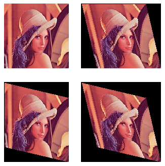
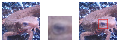
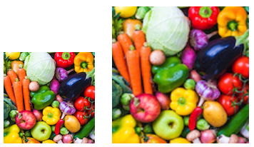
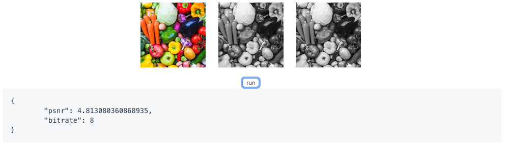
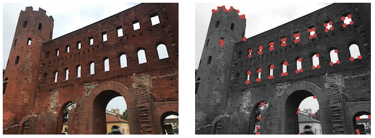
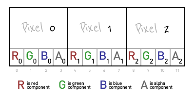
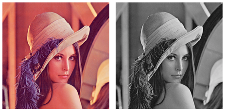
- 投稿日:2019-05-27T01:32:17+09:00
癌細胞データベース(CCLE)の癌種分類(1)
ヒト癌細胞データベース(CCLE)の解析
バイオデータセットの最低サンプル数
今回はアメリカの 「The Broad Institute」 が提供している、ヒト癌細胞の 「遺伝子発現データベース、CCLE」 の解析を行います。バイオビッグデータを解析していて困るのは、通常の機械学習と比べて 「データ数よりもパラメータ数の方が圧倒的に多いことが多い」 、ことです。
機械学習の大御所、 スタンフォード大学Andrew Ng先生の「Machine learning」講義でも触れられていますが、基本的には 「It's not who has the best algorithm that wins,It's who has the most data」 が示す通り、データ数が少ない場合は、機械学習の精度に大きく貢献するのはアルゴリズム云々よりも 「データ数」 の方です。
[Banko & Brill, 2001][Coursera:機械学習]
https://ja.coursera.org/learn/machine-learningでは 「どれくらいのデータ量が必要となるか」 、ということですが、上記の2001年の論文ではよく見るとX軸となるトレーニングデータセットのサイズの最小値が 0.1 millions(=100,000) となっています(!)。2001年当時はアルゴリズムが今ほど洗練されていなかったことを考慮しても、バイオデータセットで10万とか普通ムリ...これって機械学習的感覚からすると、よく囁かれる 「医学生物学論文の70%以上が再現できない」 のなんて当たり前じゃない?、だってデータセット(=モデル数)少なすぎるじゃん!、となる気がします。
私は元々バイオベースの人間なので、Andrew Ng先生のWeb講義受けて一番衝撃だったのが実はこのデータでした・・・この講義、個人的には全国の生物系大学の基礎学習課程で必須にした方がいいと思います。既存の堅固に見える生物学的ロジックが、数量的には砂上の楼閣に近いという感覚を初期に持つことは結構大事なんじゃないでしょうか・・・
(*最近は転移学習の研究も進んでいるため、Deep learningを用いて少数データ数の精度を上げよう、という流れもあると思うのですが、そのあたりはまだフォローしきれていません...)ただ、そうするとバイオインフォマティクスが全て終わってしまうので(笑)、気を撮り直してPythonの有名な機械学習ライブラリ、 「Scikit-learn」 のチートシートを見てみます。すると、一応ミニマムデータセットは 「50」 からに(ホッ)。
まあそれでも既存の生物研究のほとんどは(機械学習に適用するという意味では)消えてしまうのですが、今回の解析対象である 「CCLE」 は「1019」細胞なので、一応第一関門はクリアしたと個人的に納得して進めることにします(-0-)。
[Scikit-learn:機械学習チートシート]
https://scikit-learn.org/stable/tutorial/machine_learning_map/index.html
CCLEデータセットの取得
ヒト癌細胞の全遺伝子発現データセットを取得するにはCCLEのHPにアクセスし、上記左上の「Data」をクリックします。データ取得には登録が必要ですが、特に問題なく登録できます。
[CCLE:The Broad Institute]
https://portals.broadinstitute.org/ccle
そして「Data」ページの「Current Data」の項を見ると色々なデータセットがずらり・・・。
今回、遺伝子の発現情報の解析では、「RNA-seq」という手法で得られたデータを、「RSEM」というソフトウェアで解析し、「TPMカウント」にしたデータを使用します(ちなみにCCLEのLegacyデータには「Micro array」と手法で得られたデータも存在します。つまり、「遺伝子発現」と一口に言っても別種のデータが存在するんですね。これが実験科学の難しいところです)。
最近の知見では、TPMカウントは「Within-sample」(=似たような転写パターンを持つサンプル同士の比較)には良いが、「Between-sample」(=異なる転写パターンを持つサンプル同士の比較)には向いていないという話も聞きますが、私自身そこまで考慮して解析する自信がない・・・、ため、とりあえず「RPKM」よりは「TPM」の方が良いだろうという適当な感じで「TPM」データの解析を行うことにします。ちなみにこのあたりの込み入った話はチャンスがあればまた別の機会に・・・
[RNA-seq解析の手法]
https://bi.biopapyrus.jp/rnaseq/mapping/
https://bi.biopapyrus.jp/rnaseq/mapping/rsem/star-rsem-paired-rnaseq.html
https://bi.biopapyrus.jp/rnaseq/analysis/normalizaiton/tpm.htmlCCLEから取得したデータは下記の(1)〜(3)種類です。
(1)CCLE_RNAseq_rsem_genes_tpm_20180929.txt.gz
解凍後> CLE_RNAseq_rsem_genes_tpm_20180929.txt
(2)Cell_lines_annotations_20181226.txt
(3)gencode.v19.genes.v7_model.patched_contigs.gtf.gz
解凍後> gencode.v19.genes.v7_model.patched_contigs.gtfこのうち、(2)はまあ特に取得する必要はないのですが、まあ一応念の為取得してみます。
(1)が遺伝子発現情報が入っているファイル、(2)がヒト癌細胞株のアノテーション情報、(3)が各遺伝子の情報が記載されているファイルです。遺伝子ID情報の取得
このうち、まず(3)のファイルから必要な遺伝子のID情報を取得します。
awkを使っても良いのですが、なるべくPython純正でやりたいと思って 「GENCODE」 と呼ばれる、世界的にゲノム情報を集約しているグループのHPの一つを見てみると、 「gftparse」 と呼ばれるパッケージが使えるとの記述があったので今回はこれを使用してみます。[GTF Parsers in Other Programming Language(GENCODE)]
https://www.gencodegenes.org/pages/data_format.html
https://github.com/openvax/gtfparse
https://anaconda.org/bioconda/gtfparse
[参考:awk を利用した GTF ファイルの処理]
https://bi.biopapyrus.jp/rnaseq/mapping/gtf.htmlまずはターミナルでパッケージ「gtfparse」のインストール。
conda install -c bioconda gtfparseその後の解析はjupyter notebookで行います。
Pandasとgtfparseのread_gtfをimport。import pandas as pd from gtfparse import read_gtf次にダウンロード・解凍したgtfデータ(3)を読み込み、登録データの数・種類を見てみます。
df = read_gtf("gencode.v19.genes.v7_model.patched_contigs.gtf") print(df.shape) print(df.columns)(436245, 21) Index(['seqname', 'source', 'feature', 'start', 'end', 'score', 'strand', 'frame', 'gene_id', 'transcript_id', 'gene_type', 'gene_status', 'gene_name', 'transcript_type', 'transcript_status', 'transcript_name', 'level', 'havana_gene', 'exon_id', 'exon_number', 'tag'], dtype='object')データ数は非常に膨大ですが、このうち今回の解析で必要なデータは遺伝子のIDのみなので、「feature」の種類で「gene」を絞り込んだあと、「gene_id」、「gene_name」、のデータのみに集約します。
#featureの絞り込み
df_genes = df[df["feature"] == "gene"]
print(df_genes.head())
#列の絞り込み
df2 = df_genes[["gene_id","gene_name"]]
print(df2.shape)
df2.head()
df_genes.head()
#df2.head()
(56238, 2)
今回のデータセットでは遺伝子数が56238個のようですね。ちなみに、今回参照したCCLEのデータセットは少し古いゲノムをリファレンスとして使用しています。2019年5月現在、最新のヒトのリファレンスゲノムは「GRCh38」ですが、CCLEデータセットでは「GRCh37(UCSC version 19)」を使用しています。また、GENCODEとは別のグループに、リファレンスゲノム情報を集約している 「ENSEMBL」 がありますが、そこには過去にリリースされたリファレンスゲノムの一覧が記載されています。結構頻繁にリファレンスゲノムはupdateされているんですね。
例:2010年〜2014年ごろにかけたリファレンスゲノムのversionの移り変わり。
[GENCODE: release history]
https://www.gencodegenes.org/human/releases.html
[ENSEMBL: Archives]
https://www.ensembl.org/info/website/archives/assembly.html話題が逸れましたが、とりあえず上記で集約したデータをcsvファイルにしておきます。
とりあえず長くなったので今回はここまで。
(たぶん近いうちに掲載予定)次回は、今回の集約データを用いていよいよ遺伝子情報の解析を実施していく予定です。df2.to_csv("r_genome_20190526.csv")
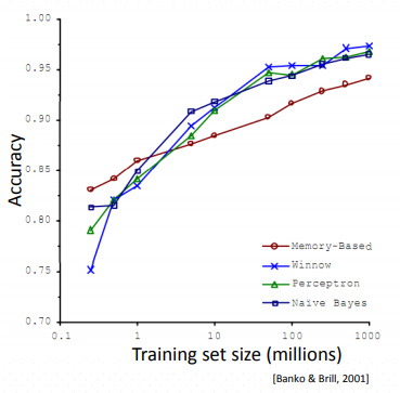
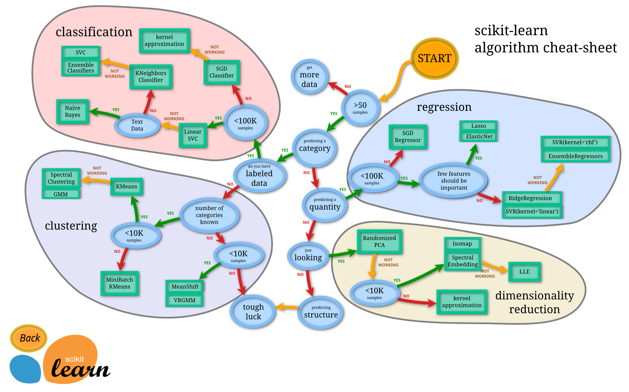

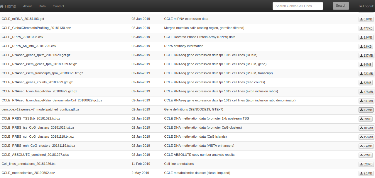


- 投稿日:2019-05-27T01:22:02+09:00
ペアノ曲線の構成法を使って一筆書きで絵を描いてみた
やったこと
ペアノ曲線、という大学で数学を学び始めた頃に出会う楽しい概念がある。ちょっと病的なところが素敵なのだ。
今回は、そのペアノ曲線の構成法とプログラミングを使って、じゃじゃっと
みたいな妙な画像(これはもちろん有名な"レナ"の画像である)を生成できるようにした。
拡大してみればわかるがこのやけに大きな画像、実は一筆書きで描かれているのである。理論的背景
ペアノ曲線(Wikipedia)とは、平面を充填する曲線の一種である(他にヒルベルト曲線Wikipediaなどがある)。
数学者のジュゼッペ・ペアノ(Wikipedia)はカントール(Wikipedia)による「線分と正方形の間の1対1写像」の発見に動機付けられて、この曲線を考えたらしい。
カントール自身も、次元の違う線分と正方形の間に1対1写像が存在することは驚きであったらしく、「理解したが、信じていない」と手紙に書いたと言われている。
しかしカントールは論文でこれが連続写像ではないことを強調することも忘れなかった。
位相に対する理解が深まった今となっては、線分と正方形が位相同型でないことを示すことは簡単な練習問題だ(1点を除いた時にどうなるか考えよ)。
当時としては、このカントールの発見こそが、集合や連続性の不思議な性質への理解を促したと言える。
そこでペアノも線分から正方形への全射な連続写像(単射ではない。当然位相同型ではない)を構成した。
それがペアノ曲線だ。
後付けの説明としては、これは(カントール集合とともに)フラクタルの先駆けにもなっている。ではペアノ曲線の構成法を見てみよう。
別にそんなに難しくない。
まず一番基本の図形がある。あとでこれを一筆書きに応用する時に、線が左上から始まる都合上最初に斜めの線で始まるが、そこは無視すれば良い。
次に、この正方形のキャンバスを9分割して、分割後のそれぞれの正方形で同じ図形を描く。
これをさらに続ける。
そしてこの操作を無限回適用し終わると、
見事に真っ黒になる、という仕掛けだ。抽象数学に現れる「極限概念」をどう応用するか
さて、ペアノ曲線は手で描いて目で見ることはできる曲線の、"極限"として定義される。
このような抽象的な議論に慣れていない方もいるかもしれないが、現代数学においてこのような"極限"による構成法に出会ったとき、多くの場合「この手法によって任意の精度が実現できる」、というように読み替えられることが多い。例えば、点列の極限についてこう読み替えれば、通常のε-N論法になる。
ただしこの読み替えは必ずしも簡単ではない。
実際、ペアノ曲線の主張に対して、正確にこのような読み替えを行うのはとても難しい。この難しさの理由は、ペアノ曲線の定義が、「空間は大きさのない点の集合として成り立っている」という点集合論に依拠しており、実はこれがそんなに理解のしやすいものではないということによると思われる。
まさにカントールが自分の証明した定理を、信じることができなかったのと根は同じである。点から空間を構成する古代ギリシャ以来の方法は「逆立ちしたやり方」であり、むしろ点は「だんだん小さくなる領域の極限」として解釈すべきものなのではないか、という見方は、実は中世スコラ哲学などにおいてもすでにみられる。
現代数学においても、「pointless topology」など、点を基礎概念としない幾何が追求されている。しかしペアノ曲線を非数学者でも扱いやすい読み替えようというのに、そのような最先端の数学が必要となっては本末転倒だ。
そこで多少情報が落ちてもいい読み替えを探るように方針を転換しよう。
そうすれば、ペアノ曲線の構成法は、「この手法によって、任意の長さ以上の一筆書きを正方形内部に収めることができる」と読み替えることが可能だ。点集合としての曲線や平面では、どこまで行っても曲線で埋められた平面の面積は0で、極限において初めて0ではなくなる。
しかし、現実世界の曲線においては、正方形の中にしめる黒の面積の割合がどんどん大きくなる。つまりペアノ曲線の理論を応用すれば、一筆書きによって任意の濃さのピクセルを表現することができるのだ。
ここまでくれば、これを応用して任意の画像を一筆書きすることができる理由もわかってきたであろう。
実装
具体的な実装は、Githubにリポジトリ(https://github.com/tannakaken/peanocurvestroke)を作ったので、それを読めばわかる。
合計200行ほどのPythonスクリプトであるし、複雑なことは全くしていないので、難しくないと思う。手順としては、
1. まず画像がカラーなら白黒にし、そのピクセルの濃さを8段階に量子化する。
2. その濃さに合わせて、ペアノ曲線の構成法で線を描き、ピクセル同士を繋いでいく。
だけである。書き捨てのスクリプトであり、非常に単純で粗雑な方法で行なっているので、工夫すればもっといい方法が見つかるかもしれない。
動作例
サンプル画像のジョゼッぺ・ペアノの肖像(パブリックドメイン)
を、このスクリプトに
./main.py Gioseppe_Peano.jpgと、この画像を入力すると、次の画像が生まれる。
一筆書きになっている様子は画像をクリックして拡大してみればわかる。
ただし、作りが雑なために、正方形にリサイズしてから処理を行っているため、アスペクト比が狂って少し横長になっている。
まあ、こんな処理で汎用ツールを作るのも馬鹿らしいので、気になるようなら、前処理をするなり、コードを書き直すなりしてほしい。
さて、こういうツールを使った時に、まずやることは、
自分の顔を入力することであろう。
見事に、火星の人面岩(光の角度でそう見えただけで、実際には少しも人面ではなかった)めいたものが出来上がった。会社ぺあのしすてむでは"数学徒"を募集している。
私の勤めている株式会社ぺあのしすてむでは、数学徒を募集している。
数学徒? なんだそりゃ、という人のために説明しよう。
数学徒とは、単に「数学を勉強しているもの」という意味だ。数学徒になるために資格は必要ないし、大学なりの機関に所属する必要もない。ただ(任意のレベルの)数学を勉強していればいいのだ(ただし、ぺあのの数学徒ポストに応募するには数学のmaster以上が必要である。悪しからず)。
数学徒が数学を活かして生きるためには二つの道がある。
1つは数学者になること、もう1つは数学屋になることだ。
数学者とは、ただ数学をしているだけで、誰かからお金をもらえる人間だ。そんな人間に私もなりたかった。
数学屋、別名数理エンジニアとは、数学を使って作った成果物を、需要を見つけて売ることによって、生計を立てる人間だ。
これらになることは、数学徒をやめることではない。
2000年以上の研究の歴史がありながら、問題が増えることはあっても減ることはなさそうな数学を前にすれば、全ての人間は永遠に数学徒であるとも言える。2019年5月27日現在、ぺあのしすてむの現在の社員は一人残らず数学徒である。
そして我々は数学屋の会社としてやっていこうと第一歩を踏み出したばかりである。我々はまた、前途ある数学徒が数学者や数学屋として生きていくことを支援したいと思っている。
数学者として生きていくことを選んだ人たちは、どこかで会社から巣立っていくのかもしれない。
数学屋として生きていくことを選んだ人たちは、我々と共に会社を盛り上げ続けてくれるのかもしれない。
先のことはわからないが、我々は数学徒が楽しく働ける会社を目指している。今回紹介したペアノ曲線の構成法による一筆書きも、学部レベルの大学数学と、ちょっとしたプログラミングができれば誰でもできる。
しかし、この程度でも結構人を驚かせることができる。
まだまだやれることはたくさん残っていることの証拠ではなかろうか。数学はArt(美しく、そして面白い)、Science(正しく、そして新しい)、Technology(強力で、便利)のいずれにも、もっと応用できる。
数学徒の皆さんは、株式会社ぺあのしすてむで、ちょっと他とは違うことをしませんか?


- 投稿日:2019-05-27T01:09:20+09:00
自分用Python備忘録
最近競プロ(AtCoder)を始めました,
もりた(Twitter)です。問題を解いたときに調べたことをメモする備忘録として随時更新してきます。(書式は情報量が増えたら整えていきます。)
count()
文字列やリストの要素を数える。
s = "abcdeeefggh"
print(s.count("e"))
#出力:3

lst = ["a", "b", "b", "c", "d"]
print(lst.count("b"))
#出力:2
min(), max()
print(min(1, 2, 3, 4, 5))
#出力:1
print(max(1, 2, 3, 4, 5))
#出力:5
print(min([1, 2, 3, 4, 5]))
#出力:1
print(max([1, 2, 3, 4, 5]))
#出力:5
複数リストの最小を求める。
先頭から順番に各リストの要素を比較して、スコアが低いほうを返す。print(min([1,2,3], [1,1,1,2])) #[1, 1, 1, 2] print(min([1,2,3], [1,2,3,4])) #[1, 2, 3] #ない要素は比較できなので、2つの要素しか比較していない #第二引数の3つ目以降がどんな要素でも関係ない print(min([1, 2], [1, 1, 3, 3, 3, 3]) #[1, 1, 3, 3, 3, 3] min([1, 2], [1, 1, 1000000]) #[1, 1, 1000000]
- 投稿日:2019-05-27T00:52:34+09:00
FLASK routineを使ってテンプレート作成【Windows.ver】
1.新規フォルダ(templetes)を作成
保存名はtemplates 複数形!(templateの単数形ではないので注意)2.templates フォルダの中に
index.htmlファイルを作成
3.index.htmlのコードは下記のように記述する
3.下記のようにrender_templateと一行目に追記することでtemplateが呼び出せる。
nameを指定する
return のところで"index.html"の後にname=value=nameを追記4.ブラウザを開くとテンプレートが表示される
さらにStep up!
index.htmlファイルの中に
{% if文 %}でpythonコードを記述できる書き方見本
{%if name_value %}
hello.pyファイルの中で
nameが指定されていたら、nameが表示される
⇒この場合はHello Flaskが表示される{% else %}
hello.pyファイルの中で
nameが指定されていなかったら
Hi, This is a penと表示される{% endif %}
if文を終了させるための命令


- 投稿日:2019-05-27T00:05:52+09:00
FLASK ~Hello Python!~と表示する【Window.Ver】
1.visual studio code に新しいフォルダ(myappという名前で保存)を作成
2.myappフォルダの中に新しいファイルを作成する(hello.pyという名前で保存)
3.下記のコードを書く
4.ターミナルに行き
Windowsの場合は
$env:FLASK="hello.py"
Flask run
5.ctrlキーを押しながら、http://127.0.0.1:5000/ を押すと
下記のようにブラウザが開きHello Python!と表示される
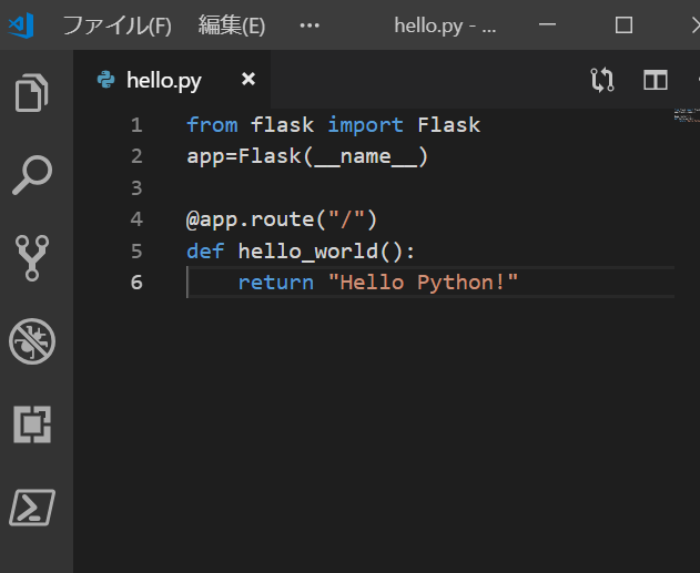
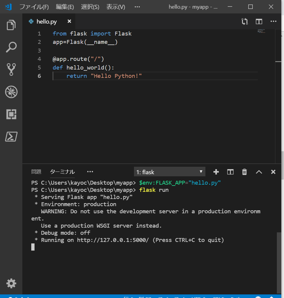

- 投稿日:2019-05-27T00:00:22+09:00
AtCoder ABC128 (Dまで)解説
カイルダイアリー(テキトー)
AtCoder Beginer Constestの解説&反省です。
使用言語はpython。A - Apple Pie
やるだけ、解説略
a,p=map(int,input().split())
print((a*3+p)//2)
B - Guidebook
c++とかだとソートがやりずらいらしい?、
でも簡単だよ、そうパイソーンならね。
速度面でc++には追い付かないので初心者さんはあまり鵜呑みにしないように、問題によって使い分けましょう。n=int(input()) q=[input().split()+[i]for i in range(n)] for i in range(n): q[i][1]=int(q[i][1]) p=sorted(sorted( q ,key=lambda x:x[1],reverse=1),key=lambda x:x[0]) for s,t,r in p: print(r+1)C - Switches
ここで会ったが100年目、bit全探索!
ABC119 Synthetic Kadomatsuの悪夢にようやく打ち勝つことができた。
最初この問題から見て意味が分からなくて発狂していたが、制約と雰囲気でなんとなくbit全探索だと分かった。
まず1~nのランプを付いてる付いてないで列挙する([t>>s&1 for s in range(n)]の部分)
そしてLに突っ込んだ、何番のスイッチと対応しているのかというのを受け取り、numpyのファンシーインデックスで何番がついているかどうかを受け取って合計し、それらを2で割った余りの配列をpと比較して同じならans+=1をするで通ります。(内包表記だと二重になってめんどいかも?)from numpy import* n,m=map(int,input().split()) l=[] for i in range(m): *a,=map(int,input().split()) l.append(a[1:]) *p,=map(int,input().split()) ans=0 for t in range(2**n): tmp=array([t>>s&1 for s in range(n)]) if p==[sum(tmp[array(i)-1])%2for i in l]: ans+=1 print(ans)D - equeue
名前の通りqueueかと思いきや、pythonだと最小値持ってくるのがないのでheapqで代用します。
まずK<nのとき、端からとれる長さfor i range(1~k)の配列を列挙します。vの後ろにvをつけることでこれは簡単に実現できます。そしてk-i回、取得した配列から最小値を捨てることができます。
(ここで手持ちがなくなっても捨てまくっていたのでREを出しまくっていました。)
一回捨てるごとにansのlistに合計を突っ込んでいきます。次にk>=nのとき、vの配列すべてを一度に取得することができ、k-n回最小値を捨てることができます。
(ここで引っ掛かったのは捨てない状態の合計をansに突っ込んでいなかったのでコーナーケースに引っかかっていました。)
同様に一回捨てるごとにansに合計を突っ込んで最後にmaxします。
これでこの問題を解くことができました。from heapq import* n,k=map(int,input().split()) *v,=map(int,input().split()) motimono=[] ans=[] if k>=n: k-=n heapify(v) ans.append(sum(v)) for i in range(k): if len(v)>0: heappop(v) ans.append(sum(v)) print(max(ans)) else: v*=2 for j in range(1,k+1): for i in range(n-j,n+1): motimono=v[i:i+j] ans.append(sum(motimono)) heapify(motimono) for i in range(k-j): if len(motimono)>0: heappop(motimono) ans.append(sum(motimono)) print(max(ans))Eからは解け次第追加します!()