20200709のTensorFlowに関する記事は2件です。

投稿日：2020-07-09T20:58:37+09:00

Tensorfrowで画像分類など学習してみる（手書き文字認識編２）

前回の記事「Tensorfrowで画像分類など学習してみる（手書き文字認識編1）」の続きになります。
前回は、MNISTデータの読み込みと、読み込んだデータの内容を確認しました。今回はその続きで、モデルを作成するまでを書いていきます。

前提/環境

前提となる環境とバージョンは下記となります。
・Anaconda3
・Python3.7.7
・pip 20.0
・TensorFlow 2.0.0

この記事ではJupyter Notebookでプログラムを進めていきます。コードの部分をJupyter Notebookにコピー＆ペーストし実行することで同様の結果が得られると思います。前回分のコードは前回の記事を参照してもらえるとありがたいです。

順伝播型ニューラルネットワークの実装

実装その3　画像データのスケール変換

読み込んだMNISTデータは下記のようなものでした。このままでは利用できないのでデータの前処理を行います。
x_train.shape: (60000, 28, 28)
x_test.shape: (10000, 28, 28)
y_train.shape: (60000,)
y_test.shape: (10000,)

画像データを変換します。28×28の2次元行列を784の1次元行列に変換します。あくまでも単に画像を1次元で扱うようにするために変換しています。
code
x_train = x_train.reshape(60000, 784) 
x_test = x_test.reshape(10000, 784) 

#変換後の構造を確認する。
print('x_train.shape:', x_train.shape)
print('x_test.shape:', x_test.shape)
結果
x_train.shape: (60000, 784)
x_test.shape: (10000, 784)

次に各ピクセルのデータを0～1の間で扱えるように変換します。
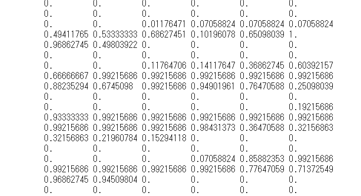
これを正規化（0～1の範囲に収める）という用語で表現します。ただし標準化と似た内容の言葉があり、場面によって標準化と表現する場合もあるようです。ここでは正規化とします。
code
x_train = x_train / 255.
x_test = x_test / 255.
1ピクセル毎の画像の濃淡を表す値が0～255までの整数で表現されているものを、0～1の間での表現に変換するということで255で割ります。

これによってどのようにデータが変換されているか確認しましょう。
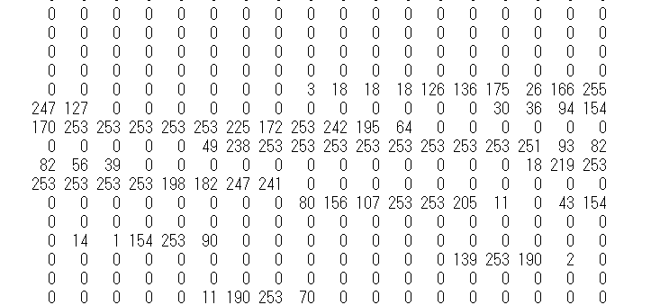
code
print(x_train[0])
結果として下記のようになります。（一部抜粋しています）
正規化前

正規化後

実装その4　ラベルデータの変換

ラベルデータについても変更します。ラベルデータは10種の0，1からなる行列に変換します。クラスラベルは整数で表現されていますが、ある値は1、その他は0で表現される形へと変換します。これを1hotベクトルといいます。
変換にはkerasのUtilsモジュールに含まれているto_categoricalメソッドを用います。
code
from tensorflow.keras.utils import to_categorical
y_train = to_categorical(y_train, 10)
y_test = to_categorical(y_test, 10)
実装その5　モデル構築

この手順でモデルを構築していきます。モデル構築ではkerasで構築する手法の一つである。Sequential APIを利用します。
code
from tensorflow.keras.models import Sequential
model = Sequential()
次のステップとして中間層を追加していきます。Denseレイヤーを用いて全結合層を追加します。全結合層はすべての入力がすべてのニューロンと結合している構造を持つ層です。
Sequential APIのaddメソッドを用いて追加します。
code
from tensorflow.keras.layers import Dense

model.add(
    Dense(
        units=64,
        input_shape=(784,),
        activation='relu'
    )
)
ここでDeneレイヤー追加時に引数を設定しています。unitsは出力する次元の数を表します。中間層として出力するニューロンの数を設定します。ここでは64としています。中間層にいくつの出力次元を設定するべきかというのは答えがありません。中間層を増やす、もっと出力次元数を大きくするなど手法はたくさんあります。結果として最終的な分類精度などを鑑みてベストな状態を探すということになります。
input_shapeは入力される行列の形を指定します。入力次元は画像のデータを一次元配列としましたが、その数である784を指定しています。
activationはそれぞれのユニットの出力時に利用する活性化関数を指定するものです。今回はreluという関数を指定します。

次のステップとして出力層を追加します。同じくDenseレイヤーをもう一つ追加します。
code
model.add(
    Dense(
        units=10,
        activation='softmax'
    )
)
ここまでで、3層の順伝播型ニューラルネットワークの準備ができました。モデルの学習のためにオプティマイザと損失関数を設定し構築します。
code
model.compile(
    optimizer='adam',
    loss='categorical_crossentropy',
    metrics=['accuracy']
)
kerasではoptimizerを指定することで最適化が可能です。今回はAdam（Adaptive Moment Estimation)を設定しています。lossは損失関数を選択します。ここでは交差エントロピーを利用します。kerasではcategorical_crossentropyなどいくつか指定ができます。
metricsは評価関数の指定をするものです。ここではaccuracyを選択しています。評価関数も種類がありますので最適なものを利用しましょう。

次回は学習を行うのと、モデルを利用して分類ができるかを試します。

　 Tweet
Qiitaで続きを読む

投稿日：2020-07-09T13:29:15+09:00

TensorFlowのバージョン1と2を比較したレシピ集（その1）

はじめに

Tensorflowはディープラーニングの代表的なフレームワークです。
このTensorFlowは2019年10月にバージョンが2.0になり、
ソースの書き方も色々変わりました。

しかし、まだまだ1.Xのバージョンで書かれた記事が大多数で、
あれ、これ2.0以降だとどう書くんだっけ？
と詰まる方も多いのではないでしょうか。

私もその1人だったので、まずは基本に立ち返ろうと備忘録がてら記事にしてみました。
色々参考にしながら自分でアレンジしていますので、
もし誤りなどございましたらコメント等いただければ幸いです。

なお、紹介するサンプルはあえて細かく説明をつけずに、
ごくシンプルにver1と2の違いの差に特化して載せております。

環境

Python 3.6.8
TensorFlow 1.15.0rc3
TensorFlow 2.1.0
Dockerで2つのコンテナを用意して検証

レシピ集

データフローグラフ

足し算

ver 1.15.0の場合

import tensorflow as tf

a = tf.constant(1, name='a')
b = tf.constant(2, name='b')
c = a + b

with tf.Session() as sess:
    print(sess.run(c))
    print(c)
    print(type(c))

out

3
Tensor("add:0", shape=(), dtype=int32)
<class 'tensorflow.python.framework.ops.Tensor'>

ver 2.1.0の場合

import tensorflow as tf

a = tf.constant(1, name='a')
b = tf.constant(2, name='b')
c = a + b

tf.print(c)
print(c)
print(type(c))

out

3
tf.Tensor(3, shape=(), dtype=int32)
<class 'tensorflow.python.framework.ops.EagerTensor'>

【参考】
tf.print

定義の出力

ver 1.15.0の場合

import tensorflow as tf

a = tf.constant(1, name='a')
b = tf.constant(2, name='b')
c = a + b

with tf.Session() as sess:
    print(sess.run(c))
    print(c)

graph = tf.get_default_graph()
print(graph.as_graph_def())

out

node {
  name: "a"
  op: "Const"
  ...(中略)...
node {
  name: "add"
  op: "AddV2"
  input: "a"
  input: "b"
  attr {
    key: "T"
    value {
      type: DT_INT32
    }
  }
}
versions {
  producer: 134
}

ver 2.1.0の場合

import tensorflow as tf

graph = tf.Graph()
with graph.as_default():
    a = tf.constant(1, name='a')
    b = tf.constant(2, name='b')
    c = a + b
    print(graph.as_graph_def())

out

# ver 1.15.0 と同様のため割愛

変数に定数を代入

ver 1.15.0の場合

import tensorflow as tf

a = tf.Variable(10, name='a')
b = tf.constant(2, name='b')
c = tf.assign(a, a + b)

with tf.Session() as sess:
    # global_variables_initializer() : 全ての変数を初期化
    sess.run(tf.global_variables_initializer())
    print(sess.run(c))
    print(sess.run(c))

out

12
14

ver 2.1.0の場合

import tensorflow as tf

a = tf.Variable(10, name='a')
b = tf.constant(2, name='b')
tf.print(a.assign_add(b))
tf.print(a.assign_add(b))

out

12
14

消えたplaceholder

ver 1.15.0の場合

import tensorflow as tf

a = tf.placeholder(dtype=tf.int32, name='a')
b = tf.constant(2, name='b')
c = a + b

with tf.Session() as sess:
    print(sess.run(c, feed_dict={a: 10}))
    print(a, b, c)

out

12
Tensor("a:0", dtype=int32) Tensor("b:0", shape=(), dtype=int32) Tensor("add:0", dtype=int32)

ver 2.1.0の場合

import tensorflow as tf

a = tf.Variable(10, name='a')
b = tf.constant(2, name='b')

# @tf.functionでAutoGraph
@tf.function
def add(x, y):
    return x + y

c = add(a,b)
tf.print(c)
print(type(c))
print(a, b, c)

out

12
<class 'tensorflow.python.framework.ops.EagerTensor'>
<tf.Variable 'a:0' shape=() dtype=int32, numpy=10> tf.Tensor(2, shape=(), dtype=int32) tf.Tensor(12, shape=(), dtype=int32)

【参考】
Migrate your TensorFlow 1 code to TensorFlow 2

四則演算

ver 1.15.0の場合

import tensorflow as tf

a = tf.constant(5, name='a')
b = tf.constant(2, name='b')
add = tf.add(a, b) # 加算
subtract = tf.subtract(a, b) # 減算
multiply = tf.multiply(a, b) # 乗算
truediv = tf.truediv(a, b) # 除算

with tf.Session() as sess:
    sess.run(tf.global_variables_initializer())
    print(sess.run(add))
    print(sess.run(subtract))
    print(sess.run(multiply))
    print(sess.run(truediv))
    print(type(add))

out

7
3
10
2.5
<class 'tensorflow.python.framework.ops.Tensor'>

ver 2.1.0の場合

import tensorflow as tf

a = tf.constant(5, name='a')
b = tf.constant(2, name='b')
add = tf.math.add(a, b) # 加算
dif = tf.math.subtract(a,b) # 減算
multiply = tf.math.multiply(a, b) # 乗算
truediv = tf.math.truediv(a, b) # 除算

tf.print(add)
tf.print(dif)
tf.print(multiply)
tf.print(truediv)
print(type(add))

out

7
3
10
2.5
<class 'tensorflow.python.framework.ops.EagerTensor'>

【参考】
tf.math

行列演算

ver 1.15.0の場合

import tensorflow as tf

a = tf.constant([[1, 2], [3, 4]], name='a')
b = tf.constant([[1], [2]], name='b')
c = tf.matmul(a, b) # 行列a, bを乗算

with tf.Session() as sess:
    print(a.shape)
    print(b.shape)
    print(c.shape)
    print('a', sess.run(a))
    print('b', sess.run(b))
    print('c', sess.run(c))

out

(2, 2)
(2, 1)
(2, 1)
a [[1 2]
 [3 4]]
b [[1]
 [2]]
c [[ 5]
 [11]]

ver 2.1.0の場合

import tensorflow as tf

a = tf.constant([[1, 2], [3, 4]], name='a')
b = tf.constant([[1], [2]], name='b')
c = tf.linalg.matmul(a, b) # 行列a, bを乗算

print(a.shape)
print(b.shape)
print(c.shape)
tf.print('a', a)
tf.print('b', b)
tf.print('c', c)

out

# ver 1.15.0 と同様のため割愛

おわりに

今回は基礎中の基礎をまとめました。
次回は勾配法など記載できたらと考えております。

　 Tweet
Qiitaで続きを読む

20200709のTensorFlowに関する記事は2件です。

Tensorfrowで画像分類など学習してみる（手書き文字認識編２）

前提/環境

順伝播型ニューラルネットワークの実装

実装その3　画像データのスケール変換

実装その4　ラベルデータの変換

実装その5　モデル構築

TensorFlowのバージョン1と2を比較したレシピ集（その1）

はじめに

環境

レシピ集

データフローグラフ

足し算

定義の出力

変数に定数を代入

消えたplaceholder

四則演算

行列演算

おわりに

日付別

タグ一覧

20200709のTensorFlowに関する記事は2件です。

Tensorfrowで画像分類など学習してみる（手書き文字認識編２）

前提/環境

順伝播型ニューラルネットワークの実装

実装その3 画像データのスケール変換

実装その4 ラベルデータの変換

実装その5 モデル構築

TensorFlowのバージョン1と2を比較したレシピ集（その1）

はじめに

環境

レシピ集

データフローグラフ

足し算

定義の出力

変数に定数を代入

消えたplaceholder

四則演算

行列演算

おわりに

日付別

タグ一覧

実装その3　画像データのスケール変換

実装その4　ラベルデータの変換

実装その5　モデル構築