1. はじめに

今学んでるディープラーニングを使って制作物を作ろうと考えました。
画像を使ったAIアプリを作れたらいいなと思い、取り組みました。

題材を何にしようか悩んでいたら父親が女子プロゴルファーにハマっていたので女子プロの診断アプリを作成しようと思った。
渋野日向子プロ、小祝さくらプロ、原英莉花プロの画像診断アプリを作ることにした。

※本当はここにも顔写真載せたかったけど著作権の関係からだめそうなので諦めました。

2. 進め方

①画像収集

②顔部分のみを取得

③不要データを削除(例えば違う顔だったり、サングラスかけてたり、なぜかおじさんの画像)

④テストデータとバリデーションデータとに分ける

⑤画像の水増し

⑥モデルの構築(今回はvgg16の転移学習)

⑦公開用のアプリケーション作成

⑧デプロイ

なかなかハードでした・・・試したこといろいろ書こうと思います。

3. 画像収集

やり方はいろいろあると思いますがicrawlerを用いました。

icrawlerとは？

Webクローラーのミニフレームワークです。画像や動画などのメディアデータをサポートしており、テキストやその他の種類のファイルにも適用可能です。Scrapyは重くて強力ですが、icrawlerは軽いみたいです。
公式リファレンス
インストール方法も載っていますのでご参考ください。

search.py

from icrawler.builtin import BingImageCrawler
import os
import shutil

# 検出する画像
golfer_lists = {'渋野日向子': 'shibuno', '小祝さくら': 'koiwai', '原英莉花': 'hara'}

# フォルダの作成
os.makedirs('./origin_image', exist_ok=True)

# keyに検索用の名前、valueはフォルダ名
for key, value in golfer_lists.items():
    # 取得した画像の保存先を指定
    crawler = BingImageCrawler(storage={'root_dir': value})
    # キーワードと取得枚数を指定
    crawler.crawl(keyword=key, max_num=1000)
    # フォルダを移動
    path = os.path.join('./', value)
    shutil.move(path, './origin_image/')

これでそれぞれ画像の取得ができました。1000枚としたけど実際は７００枚くらいでした。

4. 顔部分の取得

顔部分の取得はface_recognitionを使いました。

face_recognition.py

import cv2
from PIL import  Image
import os, glob
import numpy as np
import random
from PIL import ImageFile
import face_recognition

# 元画像が入っている大元のフォルダ
in_dir = './origin_image/*'
# 顔部分のみ取り出した画像が入る
out_dir = './face'
# 各選手のフォルダ
in_file = glob.glob(in_dir)
# 各選手のフォルダ名を取得
fileName_lists = os.listdir('./origin_image')
# テストファイルの保存先
test_image_path = './test_image/'

# 各フォルダごとに処理を行う
for golfer, fileName in zip(in_file, fileName_lists):
    # 各選手の画像リストを取得
    in_jpg = glob.glob(golfer + '/*')
    # 各選手の画像名
    in_fileName=os.listdir(golfer)
    # 各選手のフォルダーパス
    folder_path = out_dir + '/' + fileName
    # 各選手の出力フォルダを作成
    os.makedirs(folder_path, exist_ok=True)

    # 各画像について処理を行う
    for i in range(len(in_jpg)):
        # 画像を読み込む
        # image(縦, 横, 3色)
        image = face_recognition.load_image_file(str(in_jpg[i]))
        faces = face_recognition.face_locations(image)

        # 画像が存在したら([(911, 2452, 1466, 1897)])のような出力がされる
        if len(faces) > 0:
            # 取得した顔画像の中で最大の物を選ぶ((top - bottom)*(right - left)を計算)
            face_max = [(abs(faces[i][0]-faces[i][2])) * (abs(faces[i][1]-faces[i][3])) for i in range(len(faces))]
            top, right, bottom, left = faces[face_max.index(max(face_max))]

            # 顔部分の画像を抜き出す
            faceImage = image[top:bottom, left:right]

            # Image.fromarray()にndarrayを渡すとPIL.Imageが得られ、そのsave()メソッドで画像ファイルとして保存できる。
            final = Image.fromarray(faceImage)

            final = np.asarray(final.resize((64, 64)))
            final = Image.fromarray(final)

            file_path = folder_path + '/' + str(i) + '.jpg'
            final.save(file_path)
        else:
            print('No Face')

ちょっと長いですがこのようになっています。

現在のフォルダ体系の確認

これで顔部分を取得できました。
あとはひたすら１枚ずつ確認する作業・・・・
大変だけどこれが大事なんです。

5. 訓練データとバリデーションデータに分ける

訓練データ80%、バリデーションデータ20%に分ける。

split.py

# 訓練データとバリデーションデータとに分ける
import os, glob
import shutil

# 顔部分のみ取り出した画像が入る
in_dir = './face/*'
# 各選手のフォルダ ['./face/shibuno'　'./face/koiwai', './face/hara']
in_file = glob.glob(in_dir) 
# 各選手のフォルダ名を取得 ['shibuno', 'koiwai', 'hara']
fileName_lists = os.listdir('./face')
# テストファイルの保存先
test_image_path = './valid/'

# 各フォルダごとに処理を行う
for golfer, fileName in zip(in_file, fileName_lists):
    # 各選手の画像リストを取得
    in_jpg = glob.glob(golfer + '/*')
    # 各選手の画像名
    in_fileName=os.listdir(golfer)

    # validation用のデータを保存する
    test_path = test_image_path + fileName
    os.makedirs(test_path, exist_ok=True)

    # バリデーション用のフォルダへ移動する
    for i in range(len(in_jpg)//5):
        shutil.move(str(in_jpg[i]), test_path+'/')

こんな感じになっていればOK。
次に訓練データの画像の水増しを行う。

6. データのかさ増し(水増し)

画像データを集めて、取捨選択することは非常に手間がかかり大変です。(ほんとに大変でした)
そこで画像データを反転したり、ずらしたりすることで新たなデータを作り出します。

pic_add

import PIL
from keras.preprocessing.image import load_img, img_to_array, ImageDataGenerator, array_to_img
import numpy as np
import os, glob
import matplotlib.pyplot as plt
import cv2

# 元画像が入っている大元のフォルダ
in_dir = './face/*'
# 顔部分のみ取り出した画像が入る
out_dir = './face'
# 各選手のフォルダパス
in_files = glob.glob(in_dir)
# 各フォルダ名
folder_names = os.listdir('./face')

# 各選手のパスとフォルダ名
for file, name in zip(in_files, folder_names):
    # 各画像
    image_files = glob.glob(file + '/*')
    # 各ファイル名
    in_fileName = os.listdir(file)

    SAVE_DIR = './face/' + name
    # 保存先ディレクトリが存在しない場合、作成する。
    if not os.path.exists(SAVE_DIR):
        os.makedirs(SAVE_DIR)

    # 各画像それぞれに水増しを行う
    for num in range(len(image_files)):
        datagen = ImageDataGenerator(
        rotation_range=40,       # ランダムに回転する回転範囲（単位degree）
        width_shift_range=0.2,   # ランダムに水平方向に平行移動する、画像の横幅に対する割合
        height_shift_range=0.2,  # ランダムに垂直方向に平行移動する、画像の縦幅に対する割合
        shear_range=0.2,         # せん断の度合い。大きくするとより斜め方向に押しつぶされたり伸びたりしたような画像になる（単位degree）
        zoom_range=0.2,          # ランダムに画像を圧縮、拡大させる割合。最小で 1-zoomrange まで圧縮され、最大で 1+zoom_rangeまで拡大される。
        horizontal_flip=True,    # Trueを指定すると、ランダムに水平方向に反転します。
        fill_mode='nearest')

        img_array = cv2.imread(image_files[num])  # 画像読み込み
        img_array = img_array.reshape((1,) + img_array.shape)  # 4次元データに変換（flow()に渡すため）

        # flow()により、ランダム変換したイメージのバッチを作成。
        # 指定したディレクトリに生成画像を保存する。
        i = 0
        for batch in datagen.flow(img_array, batch_size=1,
                                save_to_dir=SAVE_DIR, save_prefix='add', save_format='jpg'):
            i += 1
            if i == 5:
                break  # 停止しないと無限ループ

これで訓練データの画像は１０００枚を超えた。

かなり長くなったのでモデルの作成は次回に持ち越す。

番外編としてカスケード分類器を用いた場合のコードも記載する。

※カスケード分類器について

当初カスケード分類器を用いて顔部分を取得しようとしたが文字部分や顔を取得できずにデータ量が六分の１くらいになってしまった。
一応カスケード分類器についても載せておきます
下記位リンク先より「haarcascade_frontalface_default.xml」をダウンロードしておく。

(https://github.com/opencv/opencv/tree/master/data/haarcascades)

cascade.py

import cv2
from PIL import  Image
import os, glob
import numpy as np
import random
from PIL import ImageFile

# 元画像が入っている大元のフォルダ
in_dir = './origin_image/*'
# 顔部分のみ取り出した画像が入る
out_dir = './face_image'
# 各選手のフォルダ
in_file = glob.glob(in_dir)
# 各選手のフォルダ名を取得
fileName_lists = os.listdir('./origin_image')
# テストファイルの保存先
test_image_path = './face_image/test_image/'

cascade_path = './haarcascade_frontalface_alt.xml'
face_cascade = cv2.CascadeClassifier(cascade_path)

# 各フォルダごとに処理を行う
for golfer, fileName in zip(in_file, fileName_lists):
    # 各選手の画像リストを取得
    in_jpg = glob.glob(golfer + '/*')
    # 各選手の画像名
    in_fileName=os.listdir(golfer)
    # 各選手のフォルダーパス
    folder_path = out_dir + '/' + fileName
    # 各選手の出力フォルダを作成
    os.makedirs(folder_path, exist_ok=True)

    # 各画像について処理を行う
    for i in range(len(in_jpg)):
        # 画像を読み込む
        image=cv2.imread(str(in_jpg[i]))
        # グレースケールにする
        image_gray = cv2.cvtColor(image, cv2.COLOR_BGR2GRAY)
        faces = face_cascade.detectMultiScale(image_gray, scaleFactor=1.1, minNeighbors=2, minSize=(64, 64))

        if len(faces) > 0:
            for j, face in enumerate(faces,1):
                x, y ,w, h =face
                save_img_path = folder_path + '/' + str(i) +'_' + str(j) + '.jpg'
                cv2.imwrite(save_img_path , image[y:y+h, x:x+w])
        else:
            print ('image' + str(i) + ':NoFace')

はじめに

前回の投稿で、日経225の値幅を60%の精度で予測できたら、年率48%の利益が得られるという戯言を吐いた。

そこで、Qiitaで情報収集。

まずは、以下の記事に注目。
https://qiita.com/akiraak/items/b27a5616a94cd64a8653

Accuracy =72%ってあるやん。
これを追試する。

使っている技術はTensorFlow。くだんの記事はTensorFlowを使ったコードを詳細に解説していて、ソースコードも公開されている。当方の理解はちんぷんかんぷんだが、さわって試してみることはできる。ただ、2017年の記事なので、いろいろ変わっていて動かすには苦労した。

元記事のスキーム

前日まで過去3日分の各市場（FTSE, GDAXI, HSI, N225, SSEC等）の値動きを説明変数、当日のSP500の引値を教師データとしてTensorflowで機械学習を行い、当日のSP500の前日比の符号を予測する予測器を構築し、その性能を評価している。ただし、詳細な原理とかは頭悪いんで理解できていない。

その結果が、Accuracy=70%台。

これは期待が持てる。

今回のスキーム

予測対象は1358日経レバ２倍とし、説明変数も微修正。

説明変数には、前日までのNIKKEI225、各国のインデックスだけでなく円ドルも含める。

教師ラベル：当日の1358日経レバ２倍の値幅（引け値-寄値）が上昇または下落

説明変数：
DOW30, NASDAQ_COMP, S&P500, FTSE_MIB, DAX, CAC40, HANG_SENG, usdjpy, NIKKEI225 各指標の過去３日分の終値（9×3=27次元）

モデルは元ソースのまま

入力層：[27, 50], stddev=0.0001
隠れ層1：[50, 25], stddev=0.0001
隠れ層2：[25, 2], stddev=0.0001
出力層：[2]

実験結果

学習期間 = 2014-10-30 〜 2017-10-31

評価期間 = 2017-11-22 〜 2020-07-09

学習回数：12000回

学習データによる精度の推移

1000 0.5241935
2000 0.55241936
3000 0.5510753
4000 0.5591398
5000 0.5645161
6000 0.56989247
7000 0.57123655
8000 0.56989247
9000 0.56182796
10000 0.5577957
11000 0.5591398
12000 0.56182796

評価期間での精度

評価数 =  673
上昇, 正解 =  127
下落, 正解 =  216
上昇, 不正解 =  130
下落, 不正解 =  200
Accuracy =  0.5096582466567607

損益シミュレーション（バックテスト）

上昇予想の場合：1358上場日経２倍
下落予想の場合：1357日経ダブルインバース
10,000,000円分を寄り付きで購入し、引けで売却する
2017-11-22 〜 2020-07-09まで、この方法を繰り返した場合の損益
-1,551,671円

月別損益

2017年11月： -83249円
2017年12月： -83258円
2018年1月： 341621円
2018年2月： -595994円
2018年3月： 626082円
2018年4月： -222331円
2018年5月： -332350円
2018年6月： -384622円
2018年7月： -375612円
2018年8月： 355649円
2018年9月： 472170円
2018年10月： -262912円
2018年11月： -251190円
2018年12月： 1321959円
2019年1月： 1181772円
2019年2月： -545563円
2019年3月： -427964円
2019年4月： 82859円
2019年5月： -465943円
2019年6月： -265452円
2019年7月： 96485円
2019年8月： 936343円
2019年9月： -723723円
2019年10月： -432153円
2019年11月： 396537円
2019年12月： 181781円
2020年1月： -303620円
2020年2月： -109976円
2020年3月： -3523718円
2020年4月： -35221円
2020年5月： 630419円
2020年6月： 1731269円

結果の考察

学習はできているようだけど、取り置きした評価データでの精度は、サイコロを振ったのと同レベル。当然ながら、バックテストの結果も全くダメ。

予測と全く逆の売買をすると損益は若干プラスになるようだが。。。

前日までの各国市場のインデックスから当日のNIKKEI225の寄り値を予測することは、先人たちの結果はAccuracy=0.7以上いけそうということだったが、寄り値を予測したところであまりご利益は無い。
単に寄る前に板を見たらわかることで、予測する必要すらない。

今回のスキームのように値幅を予測するということは、寄り値とその先の引値を予測しなければならない訳で、このAccuracyが0.5096ということは、そんな予測はできないということになる。当然といえば当然。寄った先は所詮ランダムウォーク。

2017/12から2020/2までは、まさにサイコロ振って売買したが如く収支トントン。
2020/2から2020/3で損失を大きくしているが、これは新型コロナ蔓延以前の平穏な状態を学習させた予測器を使用したため、コロナ渦で大きく予測を外したということが言えるのではないだろうか。

累積損益のグラフを眺めると、全期間が全くランダムではなく、いいとき（予測が当たるとき）と悪いときがまとまって存在するように見える。

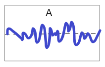
同じ収支トントンでも累積損益グラフがAのような場合と、今回のようなBのような場合とでは、予測器の質が異なるように思う。BよりもAのほうが質がいい。今回の予測器は質が悪い！

今回の予測器で、たまたま2018/12から運用を開始したとすると、最初の数か月は大儲け状態となり、「俺って天才！」と浮かれてしまい、その後の判断を誤り大やけどを負うことになってしまう。

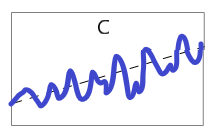
損益に大きな周期が出るような予測器Bはダメな予測器であり、小刻みにプラスを積み重ねるような予測器Cを作ることを新たな目標にするということで、今回は締めくくる。

まとめ

• 代表市場のインデックスの過去３日の引値を、翌日の日経平均の 値幅の符号を教師ラベルとして機械学習させてみたが、Accuracyが0.5096しかなく、 うまくいかなかった。
• 質の良い予測器はどんなものかの考察ができ、目標ができた。

「Yahoo! Finance.東京株式市場見通しの真贋 」につづく

日付ごとのランキングデータを元に、spotifyのデータだけを使ってランキング予測をしていきます。

今回はまず取り掛かりの第一回目として、
1.トラックごとのランキング推移をSpotifyの全期間取得
2.sklearnを使って簡易予測データ（学習データと検証データ）を作成
3.グラフで予測データを可視化

1.トラックごとのランキング推移をSpotifyの全期間取得

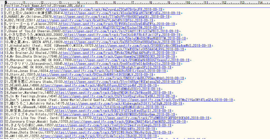
Spotifyは2017年からのデータをcsvでダウンロードできますので、そのデータを使っていきます。
2017年1月1日からのデータを一つのcsvにまとめます。

作成したファイル一覧がこちら

これで日付が入った3年半のデータが取れました。
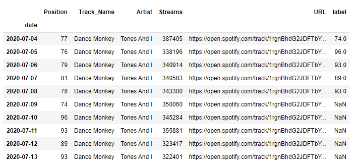
このcsvを元にまずはとある楽曲１曲を選び、ランキングがどう変化したのかグラフを作っていきます。

前回同様jupyter Notebookを使って作業していきます。
細かい詳細は省きますが、

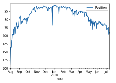
今回はTones And Iの「Dance Monkey」のランキング推移を使い、matplotで可視化しました。

https://www.youtube.com/watch?v=q0hyYWKXF0Q

今回はTones And Iの「Dance Monkey」（ https://www.youtube.com/watch?v=q0hyYWKXF0Q ）のランキング推移を使い、matplotで可視化しました。
初めてランキングにインしたのが2019年7月31日で、そこからどう推移しているかというと・・・
2019年7月31日に最初にランクインし、2020年1月に山を迎え、4月末〜降下しているのがグラフから見てとれます。

2.sklearnを使って簡易予測データ（学習データと検証データ）を作成

ここからが今回の本番。今後の予測を作っていきます。
が、本来ならSpotifyだけでは予測は難しいため、今回はかなりざっくりとした予測になります。
早速やってみましょー！

今回は統計学の中でも簡易的な株価予測にも用いられる「線形回帰（Linear regression）」という手法を使って機械学習させていきたいと思います。

まずはpandasでデータを整形し、「predict」という列を作り、順位の5日前までのデータを格納します。

学習データと検証データを8:2で分け、データの確認

やはり5日分だと精度としては少し低いですね。。

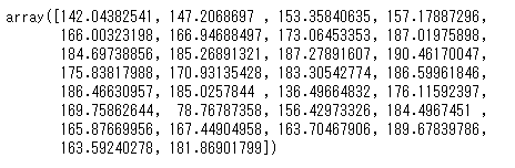
色々と試した結果、30日程度のバッファを持つと良さげな感じです。

上記スクリーンショットの「label」列のNaN部分のデータの予測がこちら。

なんとなくいいような・・グラフにしてみます。

3.グラフで予測データを可視化

なるほど、、
他要因がない限り、かなり急激に再生回数が落ちる予測になりました。。

おそらくこのままの予測どおりではなく、別要因も作用してくるはずなので一概にこの予測どおりにいくかは不明ですが、
Spotifyのデータだけでもある程度予測できるのが分かってもらえたかと思います。

次回は他データのAPIも使って同じようにプロットしていきたいと思います。

次回はより高度にランキングデータを取り、ランキング予測をしたいと思います。
ではまた！

はじめに

Google colaboratoryでTPUを使えば計算時間が短縮できるので、GPUを自前で用意できない人には強力なツールになります。しかし、TPUを扱っている記事は少なく、フレームワーク自体の変化が激しいので、調べた記事の内容に沿ってコーディングしても動かせなかったりします。一々Tensorflowのリリースノートを見てコーディングをし直すことは面倒な上、TPUの使用は控えめに言って意味不明なので、今回はとりあえず2020/07/31時点でTPUの訓練を行える方法を記します。

前準備

ColabのTPUへ接続する

import tensorflow as tf
import os
print(tf.__version__)

tpu_grpc_url = "grpc://" + os.environ["COLAB_TPU_ADDR"]
tpu_cluster_resolver = tf.distribute.cluster_resolver.TPUClusterResolver(tpu_grpc_url)
tf.config.experimental_connect_to_cluster(tpu_cluster_resolver)
tf.tpu.experimental.initialize_tpu_system(tpu_cluster_resolver)
strategy = tf.distribute.experimental.TPUStrategy(tpu_cluster_resolver)

これは、他のサイトでもよく見られるColabのTPUに接続するためのコードですが、注意点があります。まず、tensorflowのバージョンは2.2.0を用いる必要があります。2020/07/31時点で、tensorflowの最新バージョンは2.3.0ですが、以下のようなエラーが出てTPUに接続できません。これは、tensorflow 2.3.0ではTPUStrategyの前のexperimentalが外れることも考慮した上での結果です。

長いので折りたたんでいます。

INFO:tensorflow:Initializing the TPU system: grpc://10.112.235.34:8470
INFO:tensorflow:Initializing the TPU system: grpc://10.112.235.34:8470
INFO:tensorflow:Clearing out eager caches
INFO:tensorflow:Clearing out eager caches
---------------------------------------------------------------------------
InvalidArgumentError                      Traceback (most recent call last)
<ipython-input-3-95d3adc1bbd6> in <module>()
      5 tpu_cluster_resolver = tf.distribute.cluster_resolver.TPUClusterResolver(tpu_grpc_url)
      6 tf.config.experimental_connect_to_cluster(tpu_cluster_resolver)
----> 7 tf.tpu.experimental.initialize_tpu_system(tpu_cluster_resolver)
      8 strategy = tf.distribute.experimental.TPUStrategy(tpu_cluster_resolver)

3 frames
/usr/local/lib/python3.6/dist-packages/tensorflow/python/tpu/tpu_strategy_util.py in initialize_tpu_system(cluster_resolver)
    109     context.context()._clear_caches()  # pylint: disable=protected-access
    110 
--> 111     serialized_topology = output.numpy()
    112 
    113     # TODO(b/134094971): Remove this when lazy tensor copy in multi-device

/usr/local/lib/python3.6/dist-packages/tensorflow/python/framework/ops.py in numpy(self)
   1061     """
   1062     # TODO(slebedev): Consider avoiding a copy for non-CPU or remote tensors.
-> 1063     maybe_arr = self._numpy()  # pylint: disable=protected-access
   1064     return maybe_arr.copy() if isinstance(maybe_arr, np.ndarray) else maybe_arr
   1065 

/usr/local/lib/python3.6/dist-packages/tensorflow/python/framework/ops.py in _numpy(self)
   1029       return self._numpy_internal()
   1030     except core._NotOkStatusException as e:  # pylint: disable=protected-access
-> 1031       six.raise_from(core._status_to_exception(e.code, e.message), None)  # pylint: disable=protected-access
   1032 
   1033   @property

/usr/local/lib/python3.6/dist-packages/six.py in raise_from(value, from_value)

InvalidArgumentError: NodeDef expected inputs 'string' do not match 0 inputs specified; Op<name=_Send; signature=tensor:T -> ; attr=T:type; attr=tensor_name:string; attr=send_device:string; attr=send_device_incarnation:int; attr=recv_device:string; attr=client_terminated:bool,default=false; is_stateful=true>; NodeDef: {{node _Send}}

このエラーからもTPUの意味分からなさが分かりますね。

分散学習に便利なデコレータ

以下に示すコードは、「TensorFlow2.0でDistributed Trainingをいい感じにやるためのデコレーターを作った」から引用させて頂いたコードをtensorflow 2.2.0に対応させたものです。詳細はリンク先のサイトを見てください。このコードで改変した点はstrategy.experimental_run_v2をstrategy.runに変更したというだけです。

from enum import Enum

class Reduction(Enum):
    NONE = 0
    SUM = 1
    MEAN = 2
    CONCAT = 3

def distributed(*reduction_flags):
    def _decorator(fun):
        def per_replica_reduction(z, flag):
            if flag == Reduction.NONE:
                return z
            elif flag == Reduction.SUM:
                return strategy.reduce(tf.distribute.ReduceOp.SUM, z, axis=None)
            elif flag == Reduction.MEAN:
                return strategy.reduce(tf.distribute.ReduceOp.MEAN, z, axis=None)
            elif flag == Reduction.CONCAT:
                z_list = strategy.experimental_local_results(z)
                return tf.concat(z_list, axis=0)
            else:
                raise NotImplementedError()

        @tf.function
        def _decorated_fun(*args, **kwargs):
            fun_result = strategy.run(fun, args=args, kwargs=kwargs)
            if len(reduction_flags) == 0:
                assert fun_result is None
                return
            elif len(reduction_flags) == 1:
                assert type(fun_result) is not tuple and fun_result is not None
                return per_replica_reduction(fun_result, *reduction_flags)
            else:
                assert type(fun_result) is tuple
                return tuple((per_replica_reduction(fr, rf) for fr, rf in zip(fun_result, reduction_flags)))
        return _decorated_fun
    return _decorator

いろいろなモジュールのインポート

from PIL import Image
import glob
import pickle
import matplotlib.pyplot as plt
import time

import os
import numpy as np
import tensorflow as tf
from tensorflow.keras.layers import *
from tensorflow.keras.models import Model
from tensorflow.keras import backend as K

データローダの設定

今回はcifar10を用いるので、cifar10のdataloderを作ります。celebAをやってみたい人は、「TensorFlow2.0 + 無料のColab TPUでDCGANを実装した」を参考にしてください。
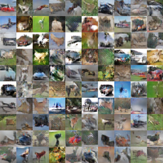
これは余談ですが、cifar10はデータ数が少なく、機械の画像や動物の画像があったりと画像ごとの違いが大きいので、頑張らないとまともな画像が生成されません。この記事ではGoogle colaboratoryのTPU分散学習をすることに重点を置いているので、生成画像はお粗末なものになっています。そこらへんはご容赦ください。
コードは以下のようになります。BATCH_SIZE=1024と非常に大きい値となっていますが、バッチサイズを大きくし、生成画像の品質が上げられるのもTPUの強みです。

def load_cifar10(batch_size):
    (x_train, y_train), (x_test, y_test) = tf.keras.datasets.cifar10.load_data()
    images = tf.concat([x_train, x_test], axis=0)
    labels = tf.concat([y_train, y_test], axis=0)
    labels = tf.keras.utils.to_categorical(labels)
    def preprocess(img):
        x = tf.cast(img, tf.float32) / 127.5 - 1.0
        return x

    dataset = tf.data.Dataset.from_tensor_slices((images, labels))
    dataset = dataset.map(
        lambda img, label: (preprocess(img), tf.cast(label, tf.float32))
    ).shuffle(4096).batch(batch_size).prefetch(tf.data.experimental.AUTOTUNE)
    return dataset

BATCH_SIZE = 1024
dataset = load_cifar10(BATCH_SIZE)

画像を表示する関数の作成

生成画像を確認するための画像を表示する関数を以下に示します。関数make_gridは「TensorFlow2.0 + 無料のColab TPUでDCGANを実装した」を引用しました。
plot_imagesに各引数（imagesはtensorflowのEagerTensorを入れる）を代入すれば使えます。
これも余談ですが、私は以前、横着してpytorchのmake_gridを使うために、tensorflowのtensorをpytorchのtensorに変換してpytorchのmake_gridを使うということを試みましたが、画像がうまく表示されませんでした。仕様もよく知らないのに横着をすると痛い目を見るということですね。

def make_grid(imgs, nrow, padding=0):
    assert imgs.ndim == 4 and nrow > 0
    batch, height, width, ch = imgs.shape
    n = nrow * (batch // nrow + np.sign(batch % nrow))
    ncol = n // nrow
    pad = np.zeros((n-batch, height, width, ch), imgs.dtype)
    x = np.concatenate([imgs, pad], axis=0)
    if padding > 0:
        x = np.pad(x, ((0, 0), (0, padding), (0, padding), (0, 0)), 
                   'constant', constant_values=(0, 0))
        height += padding
        width += padding
    x = x.reshape(ncol, nrow, height, width, ch)
    x = x.transpose([0, 2, 1, 3, 4])
    x = x.reshape(height*ncol, width*nrow, ch)
    if padding > 0:
        x = x[:(height*ncol - padding), :(width*nrow - padding), :]
    return x

def plot_images(images, nrow=10, padding=0, img_name='sample_img.png', plotting=True):
    imgs = images.numpy()
    grid = make_grid(imgs, nrow, padding)
    grid = ((grid+1)*127.5).astype(np.uint8)
    plt.figure(figsize=(10, 10))
    plt.axis('off')
    plt.imshow(grid)
    plt.savefig(img_name, bbox_inches='tight', pad_inches=0.0)
    if plotting: plt.show()
    plt.close('all')

モデルの構築

今回はGoogle colaboratoryのTPU分散学習をすることに重点を置いているので、モデルは適当に組みました。せっかくなので拙作「Colab TPUでもtensorflow.kerasでBilinear法のアップサンプリングを行う方法」のコードを用いてアップサンプリングを行いました。どれくらいの効果が合ったのかは知りません。

各関数の定義

BATCH_SIZE = 1024
Z_DIM = 512 # 潜在変数の次元

def upsampling2d_bilinear(inputs, scale=2):
    w, h = inputs.shape[1], inputs.shape[2]
    w *= scale; h *= scale
    return tf.compat.v1.image.resize_bilinear(inputs, (w, h), align_corners=True)

def ch(res):
    c = 1024*4 // res
    if c > 1024: c = 1024
    if c < 128: c = 128
    return c

Discriminatorの定義

def d_block(x, res):
    a = Conv2D(ch(res//2), kernel_size=1, use_bias=False)(x)
    a = AveragePooling2D()(a)

    x = ReLU()(x)
    x = Conv2D(ch(res), kernel_size=4, strides=2, padding='same', use_bias=False)(x)
    x = ReLU()(x)
    x = Conv2D(ch(res//2), kernel_size=4, strides=1, padding='same', use_bias=False)(x)

    x = Add()([x, a])
    return x

def create_D():
    inputs = Input((32,32,3))
    x = inputs
    for i, res in enumerate([32, 16, 8]):
        x = d_block(x, res)
    x = ReLU()(x)
    out = Conv2D(1, kernel_size=1, use_bias=False)(x)
    return Model(inputs, out)

なんとなくResidual blockを使っています。outputのサイズは(batch_size, 4, 4, 1)です。これは、Patch GANのようなものです。このあと定義するLossもそれに対応したものにしています。

Generatorの定義

def g_block(x, res):
    a = Lambda(upsampling2d_bilinear, arguments={'scale': 2})(x)
    a = Conv2D(ch(res), kernel_size=1, use_bias=False)(a)

    x = BatchNormalization()(x)
    x = ReLU()(x)
    x = Conv2DTranspose(ch(res//2), kernel_size=4, strides=2, padding='same', use_bias=False)(x)
    x = BatchNormalization()(x)
    x = ReLU()(x)
    x = Conv2D(ch(res), kernel_size=4, strides=1, padding='same', use_bias=False)(x)

    x = Add()([x, a])
    return x

def create_G():
    inputs = Input((Z_DIM,))
    x = Reshape((1, 1, Z_DIM))(inputs)
    for i, res in enumerate([8, 16, 32]):
        if i==0:
            x = Conv2DTranspose(ch(res//2), kernel_size=4, strides=1, padding='valid', use_bias=False)(x)
        else:
            x = g_block(x, res)
    x = BatchNormalization()(x)
    x = ReLU()(x)
    x = Conv2DTranspose(ch(32), kernel_size=4, strides=2, padding='same', use_bias=False)(x)
    x = BatchNormalization()(x)
    x = ReLU()(x)
    x = Conv2D(3, kernel_size=4, strides=1, padding='same', use_bias=False)(x)
    out = Activation('tanh')(x)
    return Model(inputs, out)

学習

各定数の設定

K.clear_session()

BATCH_SIZE = 1024
Z_DIM = 512
STEPS_PER_EPOCH = 60000 // BATCH_SIZE + 1

out_dir = 'out'
os.makedirs(out_dir, exist_ok=True)

ネットワーク等の定義

with strategy.scope():
    netD = create_D()
    netG = create_G()
    optD = tf.keras.optimizers.Adam(learning_rate=1e-4, beta_1=0.0, beta_2=0.9)
    optG = tf.keras.optimizers.Adam(learning_rate=1e-4, beta_1=0.0, beta_2=0.9)
    dataset = load_cifar10(BATCH_SIZE)
    dataset = strategy.experimental_distribute_dataset(dataset)

strategy.experimental_distribute_datasetによってdatasetはEagerTensorを吐き出すものからPerReplicaを吐き出すものに変わります。PerReplicaはEagerTensorのように処理できなるので注意です。

Loss関数の定義

with strategy.scope():
    class Losses:
        @staticmethod
        def hinge_loss(logits, loss_type):
            assert loss_type in ['gen', 'dis_real', 'dis_fake']
            if loss_type == 'gen':
                return -tf.reduce_mean(logits, axis=(1,2,3))
            elif loss_type == 'dis_real':
                minval = tf.minimum(logits-1, tf.zeros(logits.shape, dtype=logits.dtype))
                return -tf.reduce_mean(minval, axis=(1,2,3))
            else:
                minval = tf.minimum(-logits-1, tf.zeros(logits.shape, dtype=logits.dtype))
                return -tf.reduce_mean(minval, axis=(1,2,3))
        @staticmethod
        def cross_entropy_loss(logits, loss_type):
            p = tf.math.sigmoid(logits)
            assert loss_type in ['gen', 'dis_real', 'dis_fake']
            if loss_type == 'gen':
                loss = -tf.math.log(p)
                return tf.reduce_mean(loss, axis=(1,2,3))
            elif loss_type == 'dis_real':
                loss = -tf.math.log(p)
                return tf.reduce_mean(loss, axis=(1,2,3))
            else:
                loss = -tf.math.log(1.0-p)
                return tf.reduce_mean(loss, axis=(1,2,3))
        @staticmethod
        def generator_loss(logits_fake):
            return Losses.hinge_loss(logits_fake, 'gen')
        @staticmethod
        def discriminator_loss(logits_real, logits_fake):
            return Losses.hinge_loss(logits_real, 'dis_real') + Losses.hinge_loss(logits_fake, 'dis_fake')

このLossはPatch GANに対応しているので、logitsは4次元テンソルである必要があります。
また、このLoss関数はhinge_lossとcross_entropy_lossに対応しています。変えたいときはgenerator_lossとdiscriminator_lossを変更してください。

学習する関数の定義

with strategy.scope():
    @distributed(Reduction.SUM, Reduction.SUM, Reduction.CONCAT)
    def train_on_batch(real):
        b_size = real.shape[0]
        z = tf.random.normal((b_size, Z_DIM))
        with tf.GradientTape() as tape_D, tf.GradientTape() as tape_G:
            fake = netG(z, training=True)

        d_loss = 0.0
        for c in range(1):
            with tape_D:
                real_out = netD(real, training=True)
                fake_out = netD(fake, training=True)
                d_loss = tf.reduce_sum(Losses.discriminator_loss(real_out, fake_out)) / BATCH_SIZE
            grad_D = tape_D.gradient(d_loss, netD.trainable_weights)
            optD.apply_gradients(zip(grad_D, netD.trainable_weights))

        with tape_G:
            fake_out = netD(fake, training=False)
            g_loss = tf.reduce_sum(Losses.generator_loss(fake_out)) / BATCH_SIZE
        grad_G = tape_G.gradient(g_loss, netG.trainable_weights)
        optG.apply_gradients(zip(grad_G, netG.trainable_weights))

        return d_loss, g_loss, fake

Discriminatorの訓練の部分をfor文で囲んでいるのはSpectral NormalizationやGradient Penaltyを適用する際にDiscriminatorの訓練回数の比率を増やす必要があるから、それに適応しやすくするためです。ここで、訓練ループの前にd_loss = 0.0を入れておかないとエラーが出ます。
次に、@distributedについてReductionの種類は、分散学習で各TPUから値が戻ってくるときに、返り値にどうして欲しいかによって決まります。例えば、d_lossやg_lossの場合、既に関数の中でBATCH_SIZEで割っているので、それらを足して欲しくなります。fakeの場合、TPUから帰ってくるのは(batch_size/TPUの数, 32, 32, 3)の画像データなので、ときはbatch_sizeのところにconcatenateして欲しいです。また、何らかの評価指標の場合、TPUからの返り値を平均したいのでReduction.MEANを使います。

訓練ループ

with strategy.scope():
    losses = []
    total_step = 0
    t0 = time.time()
    EPOCH = 50
    for epoch in range(EPOCH):
        t1 = time.time()
        print(f'Epoch: {str(epoch).zfill(3)}')
        for step, (real, label) in enumerate(dataset):
            # 最後のstepでNonetypeをTensorに変換しようとしやがるのでcontinueさせる。
            if step==(STEPS_PER_EPOCH-1): continue
            d_loss, g_loss, fake = train_on_batch(real)
            if step%(STEPS_PER_EPOCH//2)==0:
                print(f'\tStep {str(total_step).zfill(7)}, d_loss: {d_loss.numpy():f}, g_loss: {g_loss.numpy():f}')
            losses.append([d_loss.numpy(), g_loss.numpy()])
            total_step += 1
        plot_images(fake[:100], img_name=f'./{out_dir}/epoch_{str(epoch).zfill(3)}.png', plotting=(epoch%2==0))
        print(f'{time.time()-t1:f}s is elapsed for epoch {str(epoch).zfill(3)}.')
    with open(f'losses.pkl', 'wb') as fp: pickle.dump(losses, fp)
    print(f'Train time: {(time.time()-t0)/60:f}min.')

if step==(STEPS_PER_EPOCH-1): continueについて、これがないとtensorflowおなじみのNoneTypeをTensorに変換しようとしたことにエラーが出ます。おそらくEpochの最後でバッチサイズに足りない分をNonetypeで送っているからだと思われます。ガバガバですね。

結果

所要時間は9.427246minでした。早いですね。

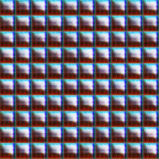
1Epoch

1Epoch目で真っ黒とか真緑とかそういう画像が生成されているときは、ほぼ訓練が失敗したと考えて良いでしょう。

10Epoch

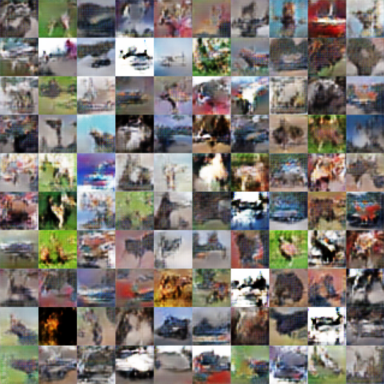
35Epoch

50Epoch

注意点

結果を見ると35Epochのほうが50Epochより画像が綺麗だと思うかも知れません。学習を進めると更に生成画像が変な画像になってきます。このことについて、以前に勾配のノルムを平均して可視化したところ、学習を進めると勾配が爆発的に大きくなるようなピークが発生しており、それによって画像の品質が劣化していると考えられます。この問題を解決するには勾配の大きさを制限するGradient Penaltyとかが非常に有効だと思われます。

はじめに

tensorflow v2.3.0 の python3.7 用の pip パッケージを Raspberry Pi zero 用にクロスビルドする。公式の手順ではビルドできないので、ビルド手順を記録しておく。

• Raspberry Pi のソースからのビルド

環境

ビルド完了までに９時間ほどかかる。

• Ubuntu 20.04
• Core i3-4030U(1.9GHz)
• Mem 16GB
• Docker 19.03.8

ビルド

TensorFlow のソースコードのダウンロード

$ git clone https://github.com/tensorflow/tensorflow.git
$ cd tensorflow
$ git checkout v2.3.0

python3.7 用の pip パッケージを作成するための変更

python 3.7 用の Docker ファイルを使用しても、python 3.7 の pip パッケージが作成できないので、cherry-pick する。

• Cannot build raspberry pi wheel for python 3.7

$ git cherry-pick 4c886a5

numpy のバージョンが 1.19 だとビルドに失敗するので、バージョン指定する。

$ vim tensorflow/tools/ci_build/install/install_pip_packages_by_version.sh

"numpy" を "numpy<1.19.0" に書き換える。

pip パッケージのみビルドするためにターゲットを変更する。
共有ライブラリが必要な場合は以下の手順は不要。

$ vim tensorflow/tools/ci_build/pi/build_raspberry_pi.sh

以下を削除する。

  //tensorflow:libtensorflow.so \
  //tensorflow:libtensorflow_framework.so \
  //tensorflow/tools/benchmark:benchmark_model \

cp bazel-bin/tensorflow/tools/benchmark/benchmark_model "${OUTDIR}"
cp bazel-bin/tensorflow/libtensorflow.so "${OUTDIR}"
cp bazel-bin/tensorflow/libtensorflow_framework.so "${OUTDIR}"

ビルド

$ CI_DOCKER_EXTRA_PARAMS="-e CI_BUILD_PYTHON=python3.7 -e CROSSTOOL_PYTHON_INCLUDE_PATH=/usr/include/python3.7" \
  tensorflow/tools/ci_build/ci_build.sh PI-PYTHON37 \
  tensorflow/tools/ci_build/pi/build_raspberry_pi.sh PI_ONE
...
...
...
Target //tensorflow/tools/pip_package:build_pip_package up-to-date:
  bazel-bin/tensorflow/tools/pip_package/build_pip_package
INFO: Elapsed time: 31682.868s, Critical Path: 485.48s
INFO: 19137 processes: 19137 local.
INFO: Build completed successfully, 24526 total actions
INFO: Build completed successfully, 24526 total actions
Final outputs will go to output-artifacts
...
Output can be found here:
output-artifacts
output-artifacts/tensorflow-2.3.0-cp37-none-linux_armv6l.whl