- 投稿日:2019-06-22T17:27:22+09:00
プログラミング完全初心者がChainerでディープラーニングを学んでみた
環境
この記事では、Python3.6以上であることが前提です。
実行はGoogle Colaboratory というサービスを利用し、ブラウザ上で実行しています。
Chainerページ: 1.はじめに-ディープラーニング入門学んだこと
はじめは
型(type)の説明があり、次に算術演算子(+,-,*,/)を学びました。
メゾット(method)やformat()、list tuple dictionaryなどもありました。
僕みたいな完全な初心者にもわかるように、一つ一つ丁寧に説明があり、とてもすすめやすかったです。
他にもif文やfor文などpythonのほぼすべてを学ぶことができるので、プログラミングが全くわからない状態でディープラーニングをやってみたいというかたにおすすめです。
- 投稿日:2019-06-22T13:06:56+09:00
3【*】Four arithmetic by Machine Learning
Qiita民が大好きなPythonで積のパーセプトロンを作成しました。
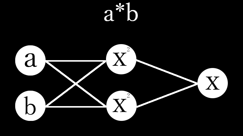
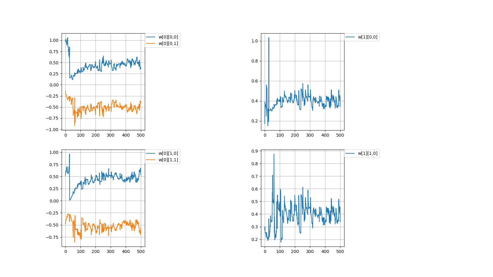
I created a perceptron of multiplication in Python which Qiita people love.# coding=utf-8 import numpy as np import matplotlib.pyplot as plt #Initial value #number of learning N = 500 #layer layer = [2, 2, 1] #bias #bias = [0.0, 0.0] #learning rate η = [1.0, 1.0] #number of middle layers H = len(η) - 1 #teacher value mul = [None for n in range(N)] #Function output value f_out = [[None for h in range(H + 1)] for n in range(N)] #Function input value f_in = [[None for h in range(H + 1)] for n in range(N)] #weight w = [[None for h in range(H + 1)] for n in range(N + 1)] for h in range(H + 1): w[0][h] = np.random.uniform(-1, 1, (layer[h], layer[h + 1])) print(w[0]) #squared error dE = [None for n in range(N)] #∂E/∂IN δ = [[None for h in range(H + 1)] for n in range(N)] #Learning for n in range(N): #Input value f_out[n][0] = np.random.uniform(-1, 1, (layer[0])) #teacher value mul[n] = f_out[n][0][0] * f_out[n][0][1] #order propagation f_in[n][0] = np.dot(f_out[n][0], w[n][0]) f_out[n][1] = f_in[n][0] * f_in[n][0] #f_out[n][1] = np.array([f_in[n][0][0] * f_in[n][0][0], -f_in[n][0][1] * f_in[n][0][1]]) #output value f_in[n][1] = np.dot(f_out[n][1], w[n][1]) #squared error dE[n] = f_in[n][1] - mul[n]#value after squared error differentiation due to omission of calculation #back propagation δ[n][1] = 1.0 * dE[n] δ[n][0] = 2.0 * f_in[n][0] * np.dot(w[n][1], δ[n][1]) #δ[n][0] = np.array([2.0 * f_in[n][0][0], -2.0 * f_in[n][0][1]]) * np.dot(w[n][1], δ[n][1]) for h in range(H + 1): w[n + 1][h] = np.array(w[n][h]) - η[h] * np.array([f_out[n][h][l] * δ[n][h] for l in range(layer[h])]) #Output #Weight print(w[N]) #Figure #weight #area height py = np.amax(layer) #area width px = (H + 1) * 2 #area size plt.figure(figsize = (16, 9)) #horizontal axis x = np.arange(0, N + 1, 1) #drawing for h in range(H + 1): for l in range(layer[h]): #area matrix plt.subplot(py, px, px * l + h * 2 + 1) for m in range(layer[h + 1]): #line plt.plot(x, np.array([w[n][h][l, m] for n in range(N + 1)]), label = "w[" + str(h) + "][" + str(l) + "," + str(m) + "]") #grid line plt.grid(True) #legend plt.legend(bbox_to_anchor = (1, 1), loc = 'upper left', borderaxespad = 0, fontsize = 10) #save plt.savefig('graph_mul.png') #show plt.show()重みの考え方を示します。 \\ I\ indicate\ the\ concept\ of\ weight. \\ \\ w[0]= \begin{pmatrix} △ & □\\ ▲ & ■ \end{pmatrix} ,w[1]= \begin{pmatrix} ○ & ● \end{pmatrix}\\ \\ 入力値とw[0]の積 \\ multiplication\ of\ input\ value\ and\ w[0]\\ w[0] \begin{pmatrix} a\\ b \end{pmatrix} = \begin{pmatrix} △ & □\\ ▲ & ■ \end{pmatrix} \begin{pmatrix} a\\ b \end{pmatrix} = \begin{pmatrix} △a + □b\\ ▲a + ■b \end{pmatrix}\\ \\ 第1層に入力\\ enter\ in\ the\ first\ layer\\ \begin{pmatrix} (△a + □b)^2\\ (▲a + ■b)^2 \end{pmatrix}\\ \\ 第1層出力とw[1]の積=出力値\\ product\ of\ first\ layer\ output\ and\ w[1]\ =\ output\ value\\ \begin{align} & w[1] \begin{pmatrix} (△a + □b)^2\\ (▲a + ■b)^2 \end{pmatrix}\\ =& \begin{pmatrix} ○ & ● \end{pmatrix} \begin{pmatrix} (a△ + b□)^2\\ (a▲ + b■)^2 \end{pmatrix}\\ =&〇(△a + □b)^2 + ●(▲a + ■b)^2\\ =&\quad (○△^2 + ●▲^2)a^2\\ &+(○□^2 + ●■^2)b^2\\\ &+(2〇△□+2●▲■)ab \end{align}\\ \\ なんだか、ややこしくなってしまってますが\\ とりあえずは、下記条件を満たせば積abを出力することができます。\\ It's\ getting\ confusing\\ For\ the\ moment,\ the\ multiplication\ ab\ can\ be\ output\ if\ the\ following\ conditions\ are\ satisfied.\\ \left\{ \begin{array}{l} ○△^2 + ●▲^2=0 \\ ○□^2 + ●■^2=0 \\ 2〇△□+2●▲■=1 \end{array} \right.毎度恒例、初期値を乱数(-1.0~1.0)の間で決めてから学習を繰り返すと目標値に収束するか試してみました。
Every time, after deciding the initial value between random numbers (-1.0~1.0),
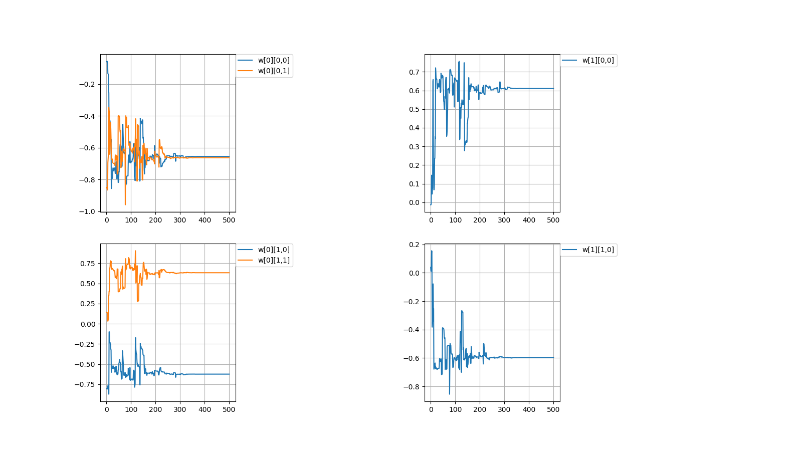
I tried to repeat the learning to converge to the target value.目標値\\ Target\ value\\ w[0]= \begin{pmatrix} △ & □\\ ▲ & ■ \end{pmatrix} ,w[1]= \begin{pmatrix} ○ & ● \end{pmatrix}\\ \left\{ \begin{array}{l} ○△^2 + ●▲^2=0 \\ ○□^2 + ●■^2=0 \\ 2〇△□+2●▲■=1 \end{array} \right. \\ 初期値\\ Initial\ value\\ w[0]= \begin{pmatrix} -0.06001642 & -0.85252436\\ -0.80560397 & 0.14216594 \end{pmatrix} w[1]= \begin{pmatrix} -0.01316071\\ 0.03798114 \end{pmatrix}\\ \left\{ \begin{array}{l} ○△^2 + ●▲^2=0.0246022702 \\ ○□^2 + ●■^2=-0.0087975322 \\ 2〇△□+2●▲■=-0.0100466654 \end{array} \right. \\ 計算値\\ Calculated\ value\\ w[0]= \begin{pmatrix} -0.65548785 & -0.66341526\\ -0.62435684 & 0.63186139 \end{pmatrix} w[1]= \begin{pmatrix} 0.61080948\\ -0.59638741 \end{pmatrix}\\ \left\{ \begin{array}{l} ○△^2 + ●▲^2=0.0299584277 \\ ○□^2 + ●■^2=0.0307223832 \\ 2〇△□+2●▲■=1.0017919987 \end{array} \right.
成功しましたが課題を抱えています。
It was successful but with challenges.1,収束する時と収束しない時がある
1,There are cases when it converges and when it doesn't converge初期値\\ Initial\ value\\ w[0]= \begin{pmatrix} 0.96898039 & -0.13805777\\ 0.5250381 & -0.457846 \end{pmatrix} w[1]= \begin{pmatrix} 0.17181768\\ 0.27522847 \end{pmatrix}\\ 計算値\\ Calculated\ value\\ w[0]= \begin{pmatrix} 0.37373305 & -0.38455151\\ 0.53163593 & -0.54773647 \end{pmatrix} w[1]= \begin{pmatrix} 0.34178043\\ 0.33940928 \end{pmatrix}\\
上記のように値が収束しない場合がときたまあります。
本当はプログラムを組んで収束しない時の統計を出すべきなんでしょうが
そこまでの気力がありませんでした。
Occasionally, the values don't converge as described above.
Properly, it should be put out the statistics when doesn't converge by programming
I didn't have the energy to get it.2,収束したらしたでいつも同じぐらいの値で収束する
どういう訳か、例えばw[0][0,0]=±0.6...ぐらいの値に落ち着く事がほとんどです。
2,It always converges with the similar value
For some reason, for example, it is almost always settled to the value of w [0][0,0] = ±0.6...一見、簡単そうなパーセプトロンでも謎が多いです。
At first glance, even the seemingly easy perceptron has many mystery.NEXT
【/】
- 投稿日:2019-06-22T13:06:56+09:00
3【*】Four Arithmetic by Machine Learning
Qiita民が大好きなPythonで積のパーセプトロンを作成しました。
I created a perceptron of multiplication in Python which Qiita people love.# coding=utf-8 import numpy as np import matplotlib.pyplot as plt #Initial value #number of learning N = 500 #layer layer = [2, 2, 1] #bias #bias = [0.0, 0.0] #learning rate η = [1.0, 1.0] #number of middle layers H = len(η) - 1 #teacher value mul = [None for n in range(N)] #Function output value f_out = [[None for h in range(H + 1)] for n in range(N)] #Function input value f_in = [[None for h in range(H + 1)] for n in range(N)] #weight w = [[None for h in range(H + 1)] for n in range(N + 1)] for h in range(H + 1): w[0][h] = np.random.uniform(-1, 1, (layer[h], layer[h + 1])) print(w[0]) #squared error dE = [None for n in range(N)] #∂E/∂IN δ = [[None for h in range(H + 1)] for n in range(N)] #Learning for n in range(N): #Input value f_out[n][0] = np.random.uniform(-1, 1, (layer[0])) #teacher value mul[n] = f_out[n][0][0] * f_out[n][0][1] #order propagation f_in[n][0] = np.dot(f_out[n][0], w[n][0]) f_out[n][1] = f_in[n][0] * f_in[n][0] #f_out[n][1] = np.array([f_in[n][0][0] * f_in[n][0][0], -f_in[n][0][1] * f_in[n][0][1]]) #output value f_in[n][1] = np.dot(f_out[n][1], w[n][1]) #squared error dE[n] = f_in[n][1] - mul[n]#value after squared error differentiation due to omission of calculation #back propagation δ[n][1] = 1.0 * dE[n] δ[n][0] = 2.0 * f_in[n][0] * np.dot(w[n][1], δ[n][1]) #δ[n][0] = np.array([2.0 * f_in[n][0][0], -2.0 * f_in[n][0][1]]) * np.dot(w[n][1], δ[n][1]) for h in range(H + 1): w[n + 1][h] = np.array(w[n][h]) - η[h] * np.array([f_out[n][h][l] * δ[n][h] for l in range(layer[h])]) #Output #Weight print(w[N]) #Figure #weight #area height py = np.amax(layer) #area width px = (H + 1) * 2 #area size plt.figure(figsize = (16, 9)) #horizontal axis x = np.arange(0, N + 1, 1) #drawing for h in range(H + 1): for l in range(layer[h]): #area matrix plt.subplot(py, px, px * l + h * 2 + 1) for m in range(layer[h + 1]): #line plt.plot(x, np.array([w[n][h][l, m] for n in range(N + 1)]), label = "w[" + str(h) + "][" + str(l) + "," + str(m) + "]") #grid line plt.grid(True) #legend plt.legend(bbox_to_anchor = (1, 1), loc = 'upper left', borderaxespad = 0, fontsize = 10) #save plt.savefig('graph_mul.png') #show plt.show()重みの考え方を示します。 \\ I\ indicate\ the\ concept\ of\ weight. \\ \\ w[0]= \begin{pmatrix} △ & □\\ ▲ & ■ \end{pmatrix} ,w[1]= \begin{pmatrix} ○ & ● \end{pmatrix}\\ \\ 入力値とw[0]の積 \\ multiplication\ of\ input\ value\ and\ w[0]\\ w[0] \begin{pmatrix} a\\ b \end{pmatrix} = \begin{pmatrix} △ & □\\ ▲ & ■ \end{pmatrix} \begin{pmatrix} a\\ b \end{pmatrix} = \begin{pmatrix} △a + □b\\ ▲a + ■b \end{pmatrix}\\ \\ 第1層に入力\\ enter\ in\ the\ first\ layer\\ \begin{pmatrix} (△a + □b)^2\\ (▲a + ■b)^2 \end{pmatrix}\\ \\ 第1層出力とw[1]の積=出力値\\ product\ of\ first\ layer\ output\ and\ w[1]\ =\ output\ value\\ \begin{align} & w[1] \begin{pmatrix} (△a + □b)^2\\ (▲a + ■b)^2 \end{pmatrix}\\ =& \begin{pmatrix} ○ & ● \end{pmatrix} \begin{pmatrix} (a△ + b□)^2\\ (a▲ + b■)^2 \end{pmatrix}\\ =&〇(△a + □b)^2 + ●(▲a + ■b)^2\\ =&\quad (○△^2 + ●▲^2)a^2\\ &+(○□^2 + ●■^2)b^2\\\ &+(2〇△□+2●▲■)ab \end{align}\\ \\ なんだか、ややこしくなってしまってますが\\ とりあえずは、下記条件を満たせば積abを出力することができます。\\ It's\ getting\ confusing\\ For\ the\ moment,\ the\ multiplication\ ab\ can\ be\ output\ if\ the\ following\ conditions\ are\ satisfied.\\ \left\{ \begin{array}{l} ○△^2 + ●▲^2=0 \\ ○□^2 + ●■^2=0 \\ 2〇△□+2●▲■=1 \end{array} \right.毎度恒例、初期値を乱数(-1.0~1.0)の間で決めてから学習を繰り返すと目標値に収束するか試してみました。
Every time, after deciding the initial value between random numbers (-1.0~1.0),
I tried to repeat the learning to converge to the target value.目標値\\ Target\ value\\ w[0]= \begin{pmatrix} △ & □\\ ▲ & ■ \end{pmatrix} ,w[1]= \begin{pmatrix} ○ & ● \end{pmatrix}\\ \left\{ \begin{array}{l} ○△^2 + ●▲^2=0 \\ ○□^2 + ●■^2=0 \\ 2〇△□+2●▲■=1 \end{array} \right. \\ 初期値\\ Initial\ value\\ w[0]= \begin{pmatrix} -0.06001642 & -0.85252436\\ -0.80560397 & 0.14216594 \end{pmatrix} w[1]= \begin{pmatrix} -0.01316071\\ 0.03798114 \end{pmatrix}\\ \left\{ \begin{array}{l} ○△^2 + ●▲^2=0.0246022702 \\ ○□^2 + ●■^2=-0.0087975322 \\ 2〇△□+2●▲■=-0.0100466654 \end{array} \right. \\ 計算値\\ Calculated\ value\\ w[0]= \begin{pmatrix} -0.65548785 & -0.66341526\\ -0.62435684 & 0.63186139 \end{pmatrix} w[1]= \begin{pmatrix} 0.61080948\\ -0.59638741 \end{pmatrix}\\ \left\{ \begin{array}{l} ○△^2 + ●▲^2=0.0299584277 \\ ○□^2 + ●■^2=0.0307223832 \\ 2〇△□+2●▲■=1.0017919987 \end{array} \right.
成功しましたが課題を抱えています。
It was successful but with challenges.1,収束する時と収束しない時がある
1,There are cases when it converges and when it doesn't converge初期値\\ Initial\ value\\ w[0]= \begin{pmatrix} 0.96898039 & -0.13805777\\ 0.5250381 & -0.457846 \end{pmatrix} w[1]= \begin{pmatrix} 0.17181768\\ 0.27522847 \end{pmatrix}\\ 計算値\\ Calculated\ value\\ w[0]= \begin{pmatrix} 0.37373305 & -0.38455151\\ 0.53163593 & -0.54773647 \end{pmatrix} w[1]= \begin{pmatrix} 0.34178043\\ 0.33940928 \end{pmatrix}\\
上記のように値が収束しない場合がときたまあります。
本当はプログラムを組んで収束しない時の統計を出すべきなんでしょうが
そこまでの気力がありませんでした。
Occasionally, the values don't converge as described above.
Properly, it should be put out the statistics when doesn't converge by programming
I didn't have the energy to get it.2,収束したらしたでいつも同じぐらいの値で収束する
どういう訳か、例えばw[0][0,0]=±0.6...ぐらいの値に落ち着く事がほとんどです。
2,It always converges with the similar value
For some reason, for example, it is almost always settled to the value of w [0][0,0] = ±0.6...一見、簡単そうなパーセプトロンでも謎が多いです。
At first glance, even the seemingly easy perceptron has many mystery.NEXT
【/】
- 投稿日:2019-06-22T08:56:23+09:00
GraphPipeが意外と使えそう
だいぶ時間が経ってしまいましたが、こちらで初めて名前を聞き、そこで紹介されたこちらでさらに説明を聞いてきたので、早速試してみました。
GraphPipeとは
Oracleが開発した、学習済みモデルを使って、簡単に推論してくれる仕組みです。
細かい話はここを見ていただくのが一番です。
また、日本語の情報としては、ABeam Consultingの澤田様がここで情報発信しています。どう簡単なの?
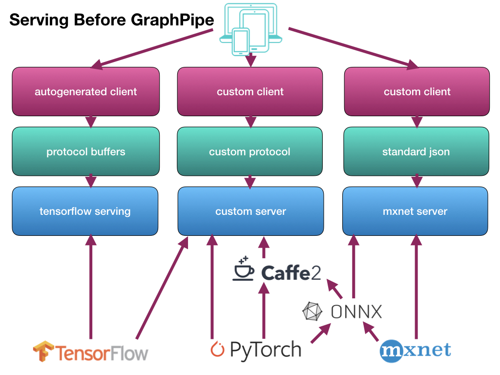
従来までの推論の流れは、それぞれのフレームワークで作成した学習済みモデルごとにサーバ側の仕組みを作成し、さらにクライアント側も合わせた形で作成していました。
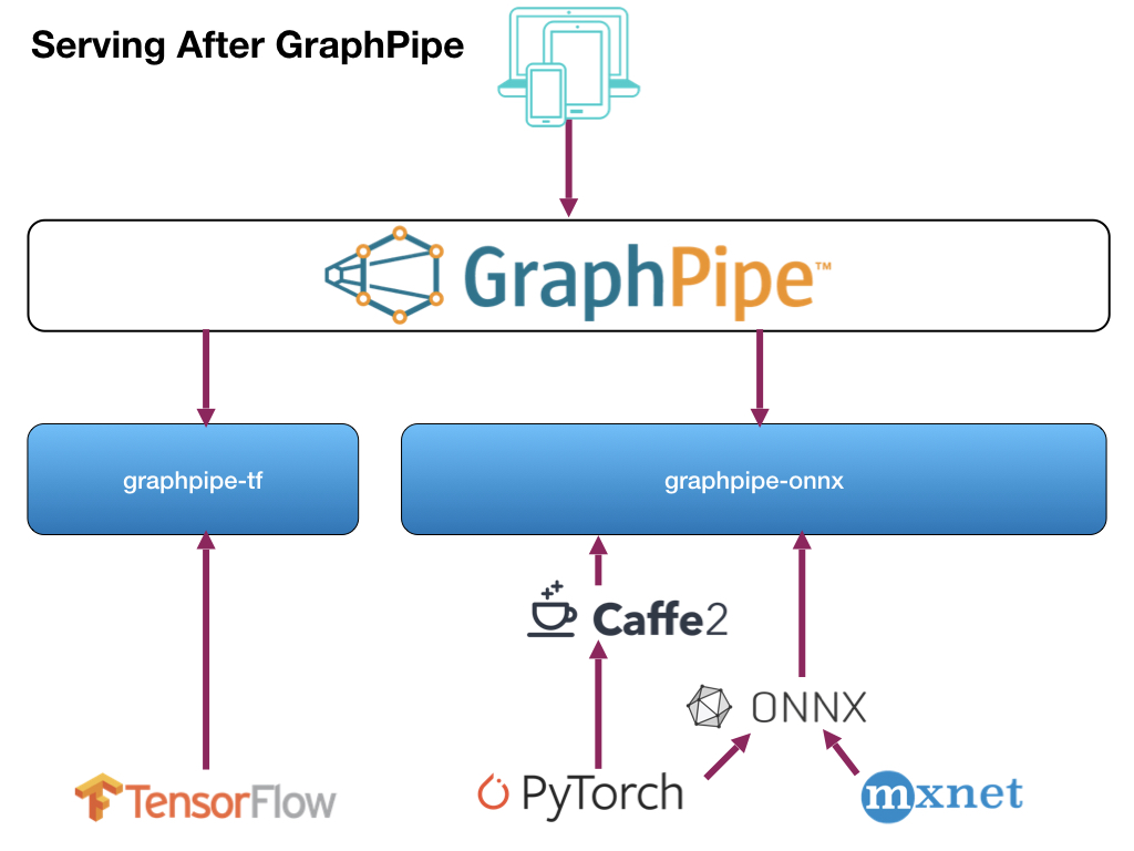
それを、サーバ側/クライアント側とも一本化(サーバ側は2つ)して、らくしましょうという仕組みです。
使い方
サーバ側/クライアント側、それぞれの使い方を見ていきます。
サーバ側
Dockerでサーバアプリを起動します。
> docker run -it --rm \ -e https_proxy=${https_proxy} \ -p 9000:9000 \ sleepsonthefloor/graphpipe-tf:cpu \ --model=https://oracle.github.io/graphpipe/models/squeezenet.pb \ --listen=0.0.0.0:9000実行するイメージは、Docker Hubから取得します。
現在、以下の6種類が用意されています。
- CPU版
- TensorFlow
- sleepsonthefloor/graphpipe-tf:cpu
- ONNX/Caffee2
- sleepsonthefloor/graphpipe-onnx:cpu
- TensorFlow+Oracle Linux
- sleepsonthefloor/graphpipe-tf:oraclelinux-cpu
- ONNX/Caffe2+Oracle Linux
- sleepsonthefloor/graphpipe-onnx:oraclelinux-cpu
- GPU版
- TensorFlow
- sleepsonthefloor/graphpipe-tf:gpu
- ONNX/Caffee2
- sleepsonthefloor/graphpipe-onnx:gpu
これらを実行するサーバ環境に合わせて選択します。
使用する学習済みモデルは、「--model」で指定します。
「--listen」でポートを指定します。クライアント側
クライアント側はPython、または、Go言語で開発ができます。
ここではPythonの場合の説明をします。準備
まずモジュールをインストールします。
> pip install grapepipeソースコードの作成
サーバとやり取りするコードを作成します。
ここでは、画像(mug227.png)を渡し、識別結果を受け取るサンプルを作成します。pred.pyfrom io import BytesIO from PIL import Image, ImageOps import numpy as np import requests from graphpipe import remote data = np.array(Image.open("mug227.png")) data = data.reshape([1] + list(data.shape)) data = np.rollaxis(data, 3, 1).astype(np.float32) # channels first print(data.shape) pred = remote.execute("http://127.0.0.1:9000", data) print(“Expected 504 (Coffee mug), got: %s” % np.argmax(pred, axis=1))実行
作成したコードを実行します。
> python pred.pyすると、すぐに結果が表示されます。
(1, 3, 227, 227)
Expected 504 (Coffe mug), got: [504]
これは、最初が送った画像のフォーマット、2行目が「正解は504で識別結果も504でした」という意味になります。
なお、実行時にはサーバ側にも実行ログが表示されます。
INFO[0491] Request for / took 195.09784msこれは、サーバ側での識別にかかった時間が195msですという意味になります。
学習済みモデルの種類
使用できる学習済みモデルは、以下のようになっています。
- TensorFlow
- SavedModel形式
- GraphDef(.pb)形式
- ONNX/Caffe2/PyTorch
- ONNX (.onnx) + value_inputs.json
- Caffe2 NetDef + value_inputs.json
Kerasの出力形式「.h5」からTensorFlowのGraphDef(.pb)への変換は、すでに用意されています。
> curl https://oracle.github.io/graphpipe/models/squeezenet.h5 > squeezenet.h5
> docker run -v $PWD:/tmp/ sleepsonthefloor/graphpipe-h5topb:latest \
  squeezenet.h5 converted_squeezenet.pb
また、Caffe2/PyTorchの場合は、それぞれONNXに変換する必要があります。
参考:GraphDef(.pb)ファイルの保存方法
import tensorflow as tf
from tensorflow.python.framework import graph_util

# グラフを構築する関数
# 学習時とも共通で使える
def build_graph():
    ...
    y = tf.nn.softmax(..., name=‘output’) # 出力層の名前

with tf.Graph().as_default() as graph:
    build_graph()

    with tf.Session() as sess:
        saver = tf.train.Saver()
        saver.restore(sess, ‘checkpoint.ckpt’) # 学習済みのグラフを読み込み

        graph_def = graph_util.convert_variables_to_constants(
            sess, graph.as_graph_def(), [‘output’]) # 出力層の名前を指定

        # プロトコルバッファ出力
        tf.train.write_graph(graph_def, '.', 'graph.pb', as_text=False)
感想
作ったモデルが簡単に検証でき、また、他の人が作ったモデルもすぐに確認できるので、非常に便利です。
データサイエンティストとアプリケーションエンジニアがお互いを意識しないで作業できるのが嬉しいです。