- 投稿日:2019-05-24T23:50:49+09:00
多項ロジスティック回帰 [TensorFlow2.0でDeep Learning 2]
(目次はこちら)
はじめに
多項ロジスティック回帰 [TensorFlowでDeep Learning 2]をtensorflow2.0で実現するためにはどうしたらいいのかを書く(
tf.keras)。コード
Python: 3.6.8, Tensorflow: 2.0.0a0で動作確認済み
多項ロジスティック回帰 [TensorFlowでDeep Learning 2] (mnist_softmax.py)を書き換えると、
v2/mnist_softmax.pyfrom helper import * IMAGE_SIZE = 28 * 28 CATEGORY_NUM = 10 LEARNING_RATE = 0.1 EPOCHS = 30 BATCH_SIZE = 100 LOG_DIR = 'log_softmax' EPS = 1e-10 def loss_fn(y_true, y): y = tf.clip_by_value(y, EPS, 1.0) return -tf.reduce_sum(y_true * tf.math.log(y), axis=1) class LR(tf.keras.layers.Layer): def __init__(self, units, *args, **kwargs): super().__init__(*args, **kwargs) self.units = units def build(self, input_shape): input_dim = int(input_shape[-1]) self.W = self.add_weight( name='weight', shape=(input_dim, self.units), initializer=tf.keras.initializers.GlorotUniform() ) self.b = self.add_weight( name='bias', shape=(self.units,), initializer=tf.keras.initializers.Zeros() ) self.built = True def call(self, x): return tf.nn.softmax(tf.matmul(x, self.W) + self.b) if __name__ == '__main__': (X_train, y_train), (X_test, y_test) = mnist_samples(flatten_image=True) model = tf.keras.models.Sequential() model.add(LR(CATEGORY_NUM, input_shape=(IMAGE_SIZE,))) model.compile(loss=loss_fn, optimizer=tf.keras.optimizers.SGD(LEARNING_RATE), metrics=['accuracy']) cb = [tf.keras.callbacks.TensorBoard(log_dir=LOG_DIR)] model.fit(X_train, y_train, batch_size=BATCH_SIZE, epochs=EPOCHS, callbacks=cb, validation_data=(X_test, y_test)) print(model.evaluate(X_test, y_test))と書ける。
ロジスティック回帰との違いは、交差エントロピーの最小化となることと、
return -tf.reduce_sum(y_true * tf.math.log(y), axis=1)
sigmoid()がsoftmax()になるくらい。return tf.nn.softmax(tf.matmul(x, self.W) + self.b)前回と同様に、シンプルに書ける。
v2/mnist_softmax_simple.pyfrom helper import * IMAGE_SIZE = 28 * 28 CATEGORY_NUM = 10 LEARNING_RATE = 0.1 EPOCHS = 30 BATCH_SIZE = 100 LOG_DIR = 'log_softmax' if __name__ == '__main__': (X_train, y_train), (X_test, y_test) = mnist_samples(flatten_image=True) model = tf.keras.models.Sequential() model.add(tf.keras.layers.Dense(CATEGORY_NUM, input_shape=(IMAGE_SIZE,), activation='softmax')) model.compile( loss='categorical_crossentropy', optimizer=tf.keras.optimizers.SGD(LEARNING_RATE), metrics=['accuracy']) cb = [tf.keras.callbacks.TensorBoard(log_dir=LOG_DIR)] model.fit(X_train, y_train, batch_size=BATCH_SIZE, epochs=EPOCHS, callbacks=cb, validation_data=(X_test, y_test)) print(model.evaluate(X_test, y_test))めでたしめでたし
- 投稿日:2019-05-24T17:33:35+09:00
最新版TensorFlow (2.0 Alpha) 画像認識編
はじめに
Tensorflow 2.0 Alpha上で画像認識サンプルを動作させた過程を記載します。
基本的にはこちらの公式チュートリアルの流れに沿って導入しています。
本記事は概要版となります。
詳細は最新版TensorFlow (2.0 Alpha) 画像認識編(詳細版)で紹介しています。
構成
MacBook Pro (13-inch, 2016, Two Thunderbolt 3 ports)
TensorFlowおよび各ライブラリの読み込み
Tensorflow 2.0 Alphaが導入されている前提で進めます。
未導入の方はこちらを参照してください:最新版TensorFlow (2.0 Alpha) 動作環境構築Tensorflowおよび各ライブラリの読み込み
from __future__ import absolute_import, division, print_function, unicode_literals

# TensorFlow and tf.keras
import tensorflow as tf
from tensorflow import keras

# Helper libraries
import numpy as np
import matplotlib.pyplot as plt

print(tf.__version__)
2.0.0-alpha0と出たらOKです。
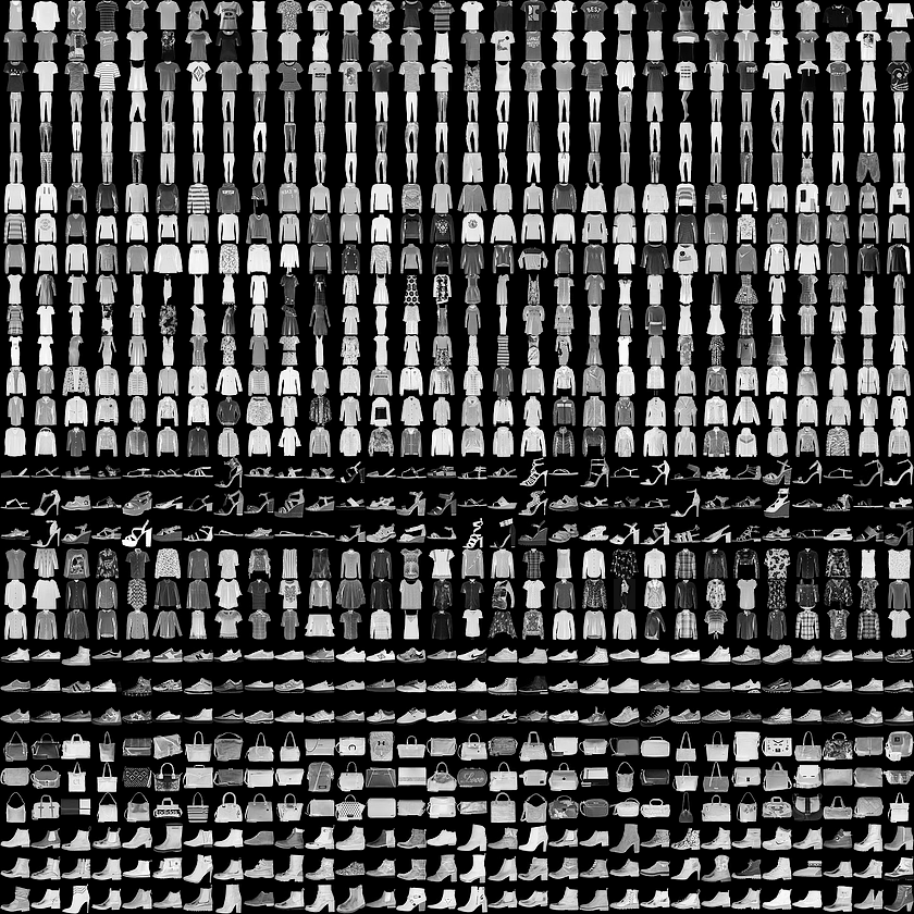
Fashion MNISTデータセットの読み込み
Fashion MNISTとは10カテゴリ計7万枚の洋服の白黒画像(28x28ピクセル)が含まれているデータセットです。
fashion_mnist = keras.datasets.fashion_mnist

(train_images, train_labels), (test_images, test_labels) = fashion_mnist.load_data()
このコマンドを入力するとダウンロードが始まります。
ラベルごとのクラス名は以下の通りです。
ラベル クラス 0 T-shirt/top 1 Trouser 2 Pullover 3 Dress 4 Coat 5 Sandal 6 Shirt 7 Sneaker 8 Bag 9 Ankle boot ただし、データセットにクラス名は含まれていないため、
以下のように設定してあげましょう。class_names = ['T-shirt/top', 'Trouser', 'Pullover', 'Dress', 'Coat','Sandal', 'Shirt', 'Sneaker', 'Bag', 'Ankle boot']データの確認
train_images.shape(60000, 28, 28)len(train_labels)60000train_labelsarray([9, 0, 0, ..., 3, 0, 5], dtype=uint8)test_images.shape(10000, 28, 28)len(test_labels)10000データの準備
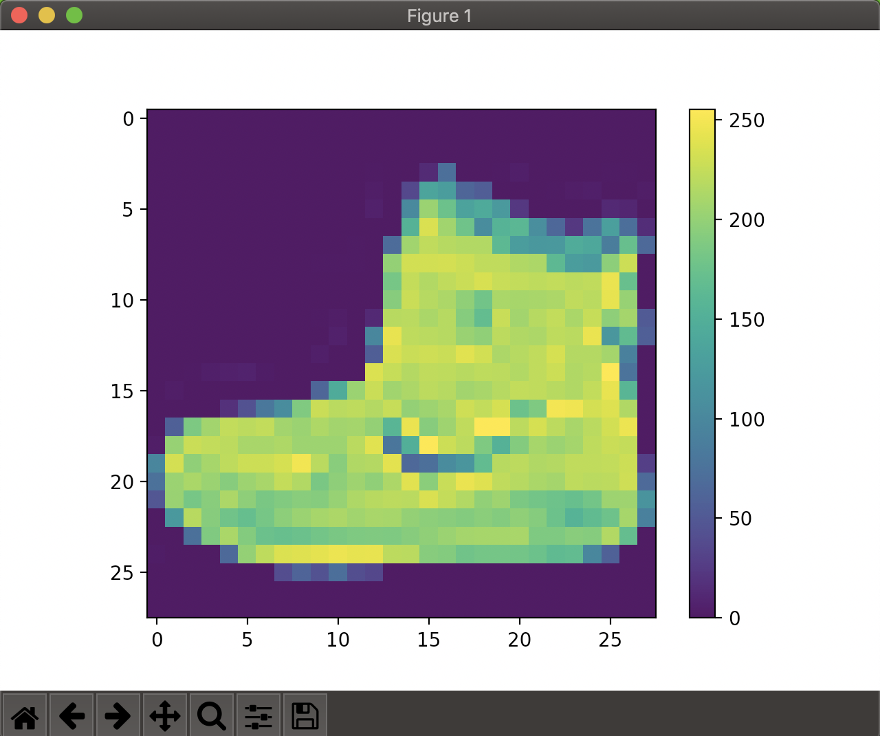
まずは画像の視覚化をしてみます。
plt.figure()
plt.imshow(train_images[0])
plt.colorbar()
plt.grid(False)
plt.show()
ウィンドウが立ち上がり、以下の画像が表示されたら成功です。
0~1の範囲にスケーリング
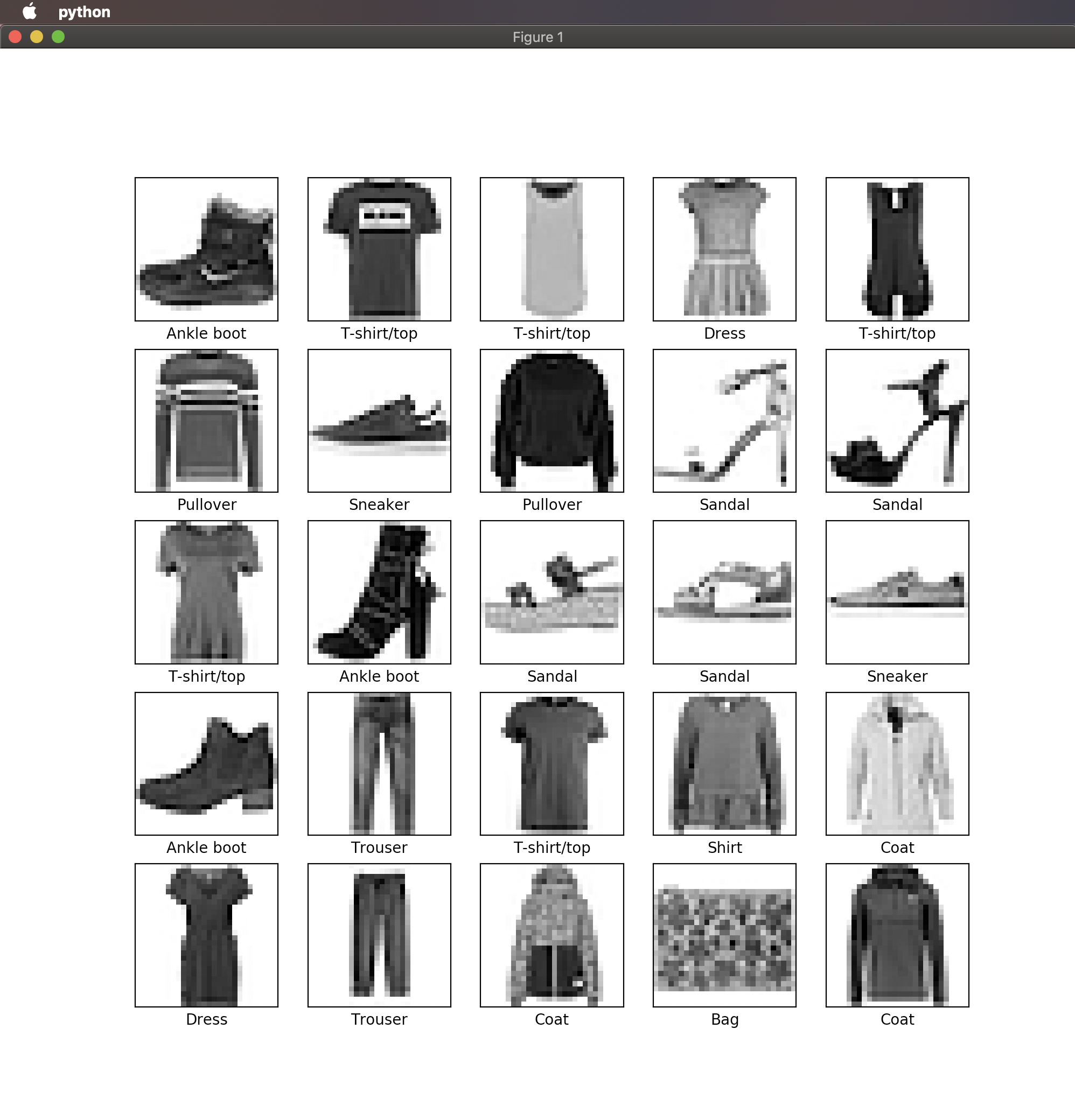
train_images = train_images / 255.0
test_images = test_images / 255.0
学習用セットの最初の25枚の画像を表示してみます。
plt.figure(figsize=(10,10))for i in range(25): plt.subplot(5,5,i+1) plt.xticks([]) plt.yticks([]) plt.grid(False) plt.imshow(train_images[i], cmap=plt.cm.binary) plt.xlabel(class_names[train_labels[i]])plt.show()
モデルの構築
いよいよ学習用モデルの構築に入ります。
model = keras.Sequential([
    keras.layers.Flatten(input_shape=(28, 28)),
    keras.layers.Dense(128, activation='relu'),
    keras.layers.Dense(10, activation='softmax')
])
モデルのコンパイル
ここでは以下のように設定しました。
model.compile(optimizer='adam',
              loss='sparse_categorical_crossentropy',
              metrics=['accuracy'])
モデルの学習
いよいよ学習を開始します。
以下のmodel.fitで訓練を開始します。
model.fit(train_images, train_labels, epochs=5)Epoch 1/5 60000/60000 [==============================] - 4s 59us/sample - loss: 1.1019 - accuracy: 0.6589 Epoch 2/5 60000/60000 [==============================] - 3s 51us/sample - loss: 0.6481 - accuracy: 0.7669 Epoch 3/5 60000/60000 [==============================] - 3s 47us/sample - loss: 0.5701 - accuracy: 0.7957 Epoch 4/5 60000/60000 [==============================] - 3s 45us/sample - loss: 0.5260 - accuracy: 0.8134 Epoch 5/5 60000/60000 [==============================] - 3s 45us/sample - loss: 0.4973 - accuracy: 0.8231 <tensorflow.python.keras.callbacks.History object at 0x11d804b70>精度としては82%程度となりました。
精度の評価
test_loss, test_acc = model.evaluate(test_images, test_labels)

print('\nTest accuracy:', test_acc)
実行結果:
Test accuracy: 0.8173学習モデルを使った予測
学習したモデルを使ってtest_imagesの予測をしてみます。
predictions = model.predict(test_images)最初の画像の予測結果を見てみます。
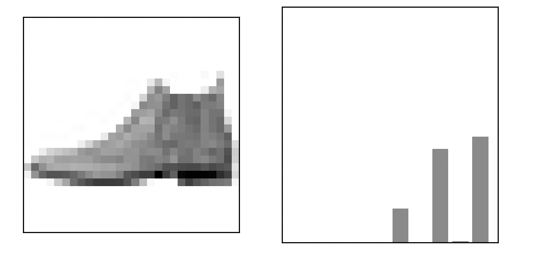
predictions[0]array([2.2446468e-06, 7.3107621e-08, 1.1268611e-05, 1.6483513e-05, 1.9317991e-05, 1.4457782e-01, 2.7507849e-05, 3.9779294e-01, 6.4411242e-03, 4.5111132e-01], dtype=float32)これは0~9のラベルに対してのそれぞれの信頼度になります。
一番信頼度が高いラベルは以下でわかります。np.argmax(predictions[0])9続いて各信頼度をグラフ化してみましょう。
def plot_image(i, predictions_array, true_label, img):
  predictions_array, true_label, img = predictions_array[i], true_label[i], img[i]
  plt.grid(False)
  plt.xticks([])
  plt.yticks([])

  plt.imshow(img, cmap=plt.cm.binary)

  predicted_label = np.argmax(predictions_array)
  if predicted_label == true_label:
    color = 'blue'
  else:
    color = 'red'

  plt.xlabel("{} {:2.0f}% ({})".format(class_names[predicted_label],
                                100*np.max(predictions_array),
                                class_names[true_label]),
                                color=color)

def plot_value_array(i, predictions_array, true_label):
  predictions_array, true_label = predictions_array[i], true_label[i]
  plt.grid(False)
  plt.xticks([])
  plt.yticks([])
  thisplot = plt.bar(range(10), predictions_array, color="#777777")
  plt.ylim([0, 1])
  predicted_label = np.argmax(predictions_array)

  thisplot[predicted_label].set_color('red')
  thisplot[true_label].set_color('blue')
最初の画像の情報を表示してみます。
i = 0
plt.figure(figsize=(6,3))
plt.subplot(1,2,1)
plot_image(i, predictions, test_labels, test_images)
plt.subplot(1,2,2)
plot_value_array(i, predictions,  test_labels)
plt.show()
まとめ
画像認識入門編としてFashion MNISTデータセットを使ったサンプル動作を一通り実現できました。
今後は、オリジナルの学習モデルの構築を目標に勉強したいと思います。
本記事は概要版となります。
詳細は最新版TensorFlow (2.0 Alpha) 画像認識編(詳細版)で紹介しています。
- 投稿日:2019-05-24T13:26:35+09:00
最新版TensorFlow (2.0 Alpha) 動作環境構築 : Mac編
はじめに
MacにTensorflow 2.0 Alphaの動作環境を構築した過程を記載します。
。
基本的にはこちらの公式チュートリアルの流れに沿って導入しています。
本記事は概要版となります。
詳細は最新版TensorFlow (2.0 Alpha) 動作環境構築 : Mac編(詳細版)で紹介しています。
構成
MacBook Pro (13-inch, 2016, Two Thunderbolt 3 ports)
TensorFlowインストール事前準備
アプリケーション→ユーティリティ→ターミナル.appを開き、以下を1行ずつ実行してください。
Python諸々のバージョン確認
python3 --version
pip3 --version
virtualenv --version
なお、現時点(2019/5/24)での私の環境では以下の通りになりました。
Python 3.7.3
pip 19.0.3
virtualenv 16.6.0仮想環境の作成(推奨)
Mac本体のシステムから独立した環境を構築したほうが、色々といじるのに便利なため、virtualenvというツールを使った仮想環境の導入をします。
virtualenv --system-site-packages -p python3 ./venvsource ./venv/bin/activatepip install --upgrade pip pip list # 仮想環境内でインストールされているパッケージを表示仮想環境を終了する場合は以下を実行してください。
なおTensorFlow使用時は有効になっている必要があります。deactivateTensorFlow 2.0 Alpha導入
以下コマンドを実行するとインストールが開始されます。
pip install --upgrade tensorflow==2.0.0-alpha0動作確認
以下を入力し対話モードに入ります。
pythonTensorflowをtfとして読み込みます。
import tensorflow as tf手書き数字のデータセットであるMNISTを読み込みます。
mnist = tf.keras.datasets.mnist

(x_train, y_train), (x_test, y_test) = mnist.load_data()
x_train, x_test = x_train / 255.0, x_test / 255.0
tf.keras.Sequentialモデルをビルドします。
model = tf.keras.models.Sequential([
  tf.keras.layers.Flatten(input_shape=(28, 28)),
  tf.keras.layers.Dense(128, activation='relu'),
  tf.keras.layers.Dropout(0.2),
  tf.keras.layers.Dense(10, activation='softmax')
])

model.compile(optimizer='adam',
              loss='sparse_categorical_crossentropy',
              metrics=['accuracy'])
学習と評価を行います。
model.fit(x_train, y_train, epochs=5)

model.evaluate(x_test, y_test)
このような感じで学習と評価がなされていれば導入完了です。
>>> model.fit(x_train, y_train, epochs=5)
Epoch 1/5
60000/60000 [==============================] - 4s 59us/sample - loss: 0.3015 - accuracy: 0.9122
Epoch 2/5
60000/60000 [==============================] - 3s 54us/sample - loss: 0.1462 - accuracy: 0.9564
Epoch 3/5
60000/60000 [==============================] - 3s 54us/sample - loss: 0.1100 - accuracy: 0.9662
Epoch 4/5
60000/60000 [==============================] - 3s 57us/sample - loss: 0.0910 - accuracy: 0.9722
Epoch 5/5
60000/60000 [==============================] - 3s 53us/sample - loss: 0.0765 - accuracy: 0.9760
<tensorflow.python.keras.callbacks.History object at 0x1123d6748>
>>>
>>> model.evaluate(x_test, y_test)
10000/10000 [==============================] - 0s 32us/sample - loss: 0.0730 - accuracy: 0.9781
[0.07304580859981943, 0.9781]
まとめ
TensorFlow 2.0 Alphaの導入、サンプル動作まで一通り実現できました。
今後は、オリジナルの学習モデルの構築を目標に勉強したいと思います。
本記事は概要版となります。
詳細は最新版TensorFlow (2.0 Alpha) 動作環境構築 : Mac編(詳細版)で紹介しています。
- 投稿日:2019-05-24T11:11:38+09:00
tensorflow2.0の学習を、gradient tapeで書くと遅い
結論はタイトルの通りです。
公式のコードを動かすだけで結果を比較できます。
今後の高速化に期待ですかね。。。Kerasのfitで学習したMNIST: https://www.tensorflow.org/alpha/tutorials/quickstart/beginner
gradient tapeで学習したMNIST: https://www.tensorflow.org/alpha/tutorials/quickstart/advanced速度結果
- kerasのfitの方が、約25倍速い。
Kerasのfit
CPU times: user 38.7 s, sys: 2.61 s, total: 41.3 s
Wall time: 30.8 s
gradient tape
CPU times: user 24min 29s, sys: 21.2 s, total: 24min 50s
Wall time: 12min 40s
その他の結果
Kerasのfit
- code
model.fit(x_train, y_train, epochs=5)

model.evaluate(x_test, y_test)
- 精度
...
Epoch 5/5
60000/60000 [==============================] - 6s 100us/sample - loss: 0.0254 - accuracy: 0.9912
10000/10000 [==============================] - 0s 44us/sample - loss: 0.0842 - accuracy: 0.9812
gradient tape
- code
@tf.function
def train_step(images, labels):
  with tf.GradientTape() as tape:
    predictions = model(images)
    loss = loss_object(labels, predictions)
  gradients = tape.gradient(loss, model.trainable_variables)
  optimizer.apply_gradients(zip(gradients, model.trainable_variables))

  train_loss(loss)
  train_accuracy(labels, predictions)

@tf.function
def test_step(images, labels):
  predictions = model(images)
  t_loss = loss_object(labels, predictions)

  test_loss(t_loss)
  test_accuracy(labels, predictions)

EPOCHS = 5

for epoch in range(EPOCHS):
  for images, labels in train_ds:
    train_step(images, labels)

  for test_images, test_labels in test_ds:
    test_step(test_images, test_labels)

  template = 'Epoch {}, Loss: {}, Accuracy: {}, Test Loss: {}, Test Accuracy: {}'
  print (template.format(epoch+1,
                         train_loss.result(),
                         train_accuracy.result()*100,
                         test_loss.result(),
                         test_accuracy.result()*100))
- 精度
Epoch 5, Loss: 0.02371377870440483, Accuracy: 99.28133392333984, Test Loss: 0.07314498722553253, Test Accuracy: 98.22599792480469考察
- Q: お手本のモデルの定義がいけないのではないか?: https://github.com/tensorflow/tensorflow/issues/23014
- A: お手本のモデルはkerasのlayerを使っているので、そこが問題では無いと考えられる。
- 投稿日:2019-05-24T11:11:38+09:00
tensorflow2.0の学習を、gradient tapeで書くと遅い?
結論はタイトルの通りです。
公式のコードを動かすだけで結果を比較できます。
今後の高速化に期待ですかね。。。Kerasのfitで学習したMNIST: https://www.tensorflow.org/alpha/tutorials/quickstart/beginner
gradient tapeで学習したMNIST: https://www.tensorflow.org/alpha/tutorials/quickstart/advanced速度結果
- kerasのfitの方が、約25倍速い。
Kerasのfit
CPU times: user 38.7 s, sys: 2.61 s, total: 41.3 s
Wall time: 30.8 s
gradient tape
CPU times: user 24min 29s, sys: 21.2 s, total: 24min 50s
Wall time: 12min 40s
その他の結果
Kerasのfit
- code
model.fit(x_train, y_train, epochs=5)

model.evaluate(x_test, y_test)
- 精度
...
Epoch 5/5
60000/60000 [==============================] - 6s 100us/sample - loss: 0.0254 - accuracy: 0.9912
10000/10000 [==============================] - 0s 44us/sample - loss: 0.0842 - accuracy: 0.9812
gradient tape
- code
@tf.function
def train_step(images, labels):
  with tf.GradientTape() as tape:
    predictions = model(images)
    loss = loss_object(labels, predictions)
  gradients = tape.gradient(loss, model.trainable_variables)
  optimizer.apply_gradients(zip(gradients, model.trainable_variables))

  train_loss(loss)
  train_accuracy(labels, predictions)

@tf.function
def test_step(images, labels):
  predictions = model(images)
  t_loss = loss_object(labels, predictions)

  test_loss(t_loss)
  test_accuracy(labels, predictions)

EPOCHS = 5

for epoch in range(EPOCHS):
  for images, labels in train_ds:
    train_step(images, labels)

  for test_images, test_labels in test_ds:
    test_step(test_images, test_labels)

  template = 'Epoch {}, Loss: {}, Accuracy: {}, Test Loss: {}, Test Accuracy: {}'
  print (template.format(epoch+1,
                         train_loss.result(),
                         train_accuracy.result()*100,
                         test_loss.result(),
                         test_accuracy.result()*100))
- 精度
Epoch 5, Loss: 0.02371377870440483, Accuracy: 99.28133392333984, Test Loss: 0.07314498722553253, Test Accuracy: 98.22599792480469考察
- Q: お手本のモデルの定義がいけないのではないか?: https://github.com/tensorflow/tensorflow/issues/23014
A: お手本のモデルはkerasのlayerを使っているので、そこが問題では無いと考えられる。
以下のissueのコードを実行すると、異なった結果がでる。(gradient_clipの方が速い)
https://github.com/tensorflow/tensorflow/issues/28714Start of epoch 0 Start of epoch 1 Start of epoch 2 Start of epoch 0 Start of epoch 1 Start of epoch 2 train 6.240314280999883 Epoch 1/3 782/782 [==============================] - 3s 4ms/step - loss: 0.3294 - sparse_categorical_accuracy: 0.9058 Epoch 2/3 782/782 [==============================] - 3s 4ms/step - loss: 0.1495 - sparse_categorical_accuracy: 0.9556 Epoch 3/3 782/782 [==============================] - 3s 3ms/step - loss: 0.1093 - sparse_categorical_accuracy: 0.9672 fit 9.801731540999754
- 投稿日:2019-05-24T11:11:38+09:00
tensorflow2.0の学習を、gradient tapeで書くと遅いと思ったがそんなことはなかった
公式のコードを動かすだけで結果を比較してしまったが故に、gradient tapeが遅いと思いましたが、そんなことはありませんでした。ほとんど同じ速度です。
Kerasのfitで学習したMNIST: https://www.tensorflow.org/alpha/tutorials/quickstart/beginner
gradient tapeで学習したMNIST: https://www.tensorflow.org/alpha/tutorials/quickstart/advanced結果
ほとんど同じでした。
Kerasのfit
Epoch 5/5
train: 60000/60000 [==============================] - 135s 2ms/sample - loss: 0.0032 - accuracy: 0.9990
test: 10000/10000 [==============================] - 6s 609us/sample - loss: 0.0890 - accuracy: 0.9823
CPU times: user 10min 35s, sys: 14.7 s, total: 10min 50s
Wall time: 11min 27s
gradient tape
Epoch 5, Loss: 0.025853322818875313, Accuracy: 99.20600128173828, Test Loss: 0.06388840824365616, Test Accuracy: 98.29166412353516
CPU times: user 22min 22s, sys: 31.7 s, total: 22min 54s
Wall time: 11min 47s
間違えた理由
- 学習しているモデルとデータが微妙に違いました。
- モデルとデータを揃えた結果、上記のようにほとんど同じ結果になりました。
参考:誤った結果(当初の間違え)
公式速度結果
- kerasのfitの方が、約25倍速い。
Kerasのfit
CPU times: user 38.7 s, sys: 2.61 s, total: 41.3 s
Wall time: 30.8 s
gradient tape
CPU times: user 24min 29s, sys: 21.2 s, total: 24min 50s
Wall time: 12min 40s
その他の結果
Kerasのfit
- code
model.fit(x_train, y_train, epochs=5)

model.evaluate(x_test, y_test)
- 精度
...
Epoch 5/5
60000/60000 [==============================] - 6s 100us/sample - loss: 0.0254 - accuracy: 0.9912
10000/10000 [==============================] - 0s 44us/sample - loss: 0.0842 - accuracy: 0.9812
gradient tape
- code
@tf.function
def train_step(images, labels):
  with tf.GradientTape() as tape:
    predictions = model(images)
    loss = loss_object(labels, predictions)
  gradients = tape.gradient(loss, model.trainable_variables)
  optimizer.apply_gradients(zip(gradients, model.trainable_variables))

  train_loss(loss)
  train_accuracy(labels, predictions)

@tf.function
def test_step(images, labels):
  predictions = model(images)
  t_loss = loss_object(labels, predictions)

  test_loss(t_loss)
  test_accuracy(labels, predictions)

EPOCHS = 5

for epoch in range(EPOCHS):
  for images, labels in train_ds:
    train_step(images, labels)

  for test_images, test_labels in test_ds:
    test_step(test_images, test_labels)

  template = 'Epoch {}, Loss: {}, Accuracy: {}, Test Loss: {}, Test Accuracy: {}'
  print (template.format(epoch+1,
                         train_loss.result(),
                         train_accuracy.result()*100,
                         test_loss.result(),
                         test_accuracy.result()*100))
- 精度
Epoch 5, Loss: 0.02371377870440483, Accuracy: 99.28133392333984, Test Loss: 0.07314498722553253, Test Accuracy: 98.22599792480469その他メモ
- Q: お手本のモデルの定義がいけないのではないか?: https://github.com/tensorflow/tensorflow/issues/23014
A: お手本のモデルはkerasのlayerを使っているので、そこが問題では無いと考えられる。
以下のissueのコードを実行すると、異なった結果がでる。(gradient_clipの方が速い)
https://github.com/tensorflow/tensorflow/issues/28714Start of epoch 0 Start of epoch 1 Start of epoch 2 Start of epoch 0 Start of epoch 1 Start of epoch 2 train 6.240314280999883 Epoch 1/3 782/782 [==============================] - 3s 4ms/step - loss: 0.3294 - sparse_categorical_accuracy: 0.9058 Epoch 2/3 782/782 [==============================] - 3s 4ms/step - loss: 0.1495 - sparse_categorical_accuracy: 0.9556 Epoch 3/3 782/782 [==============================] - 3s 3ms/step - loss: 0.1093 - sparse_categorical_accuracy: 0.9672 fit 9.801731540999754