- 投稿日:2019-05-24T23:50:49+09:00
多項ロジスティック回帰 [TensorFlow2.0でDeep Learning 2]
(目次はこちら)
はじめに
多項ロジスティック回帰 [TensorFlowでDeep Learning 2]をtensorflow2.0で実現するためにはどうしたらいいのかを書く(
tf.keras)。コード
Python: 3.6.8, Tensorflow: 2.0.0a0で動作確認済み
多項ロジスティック回帰 [TensorFlowでDeep Learning 2] (mnist_softmax.py)を書き換えると、
v2/mnist_softmax.pyfrom helper import * IMAGE_SIZE = 28 * 28 CATEGORY_NUM = 10 LEARNING_RATE = 0.1 EPOCHS = 30 BATCH_SIZE = 100 LOG_DIR = 'log_softmax' EPS = 1e-10 def loss_fn(y_true, y): y = tf.clip_by_value(y, EPS, 1.0) return -tf.reduce_sum(y_true * tf.math.log(y), axis=1) class LR(tf.keras.layers.Layer): def __init__(self, units, *args, **kwargs): super().__init__(*args, **kwargs) self.units = units def build(self, input_shape): input_dim = int(input_shape[-1]) self.W = self.add_weight( name='weight', shape=(input_dim, self.units), initializer=tf.keras.initializers.GlorotUniform() ) self.b = self.add_weight( name='bias', shape=(self.units,), initializer=tf.keras.initializers.Zeros() ) self.built = True def call(self, x): return tf.nn.softmax(tf.matmul(x, self.W) + self.b) if __name__ == '__main__': (X_train, y_train), (X_test, y_test) = mnist_samples(flatten_image=True) model = tf.keras.models.Sequential() model.add(LR(CATEGORY_NUM, input_shape=(IMAGE_SIZE,))) model.compile(loss=loss_fn, optimizer=tf.keras.optimizers.SGD(LEARNING_RATE), metrics=['accuracy']) cb = [tf.keras.callbacks.TensorBoard(log_dir=LOG_DIR)] model.fit(X_train, y_train, batch_size=BATCH_SIZE, epochs=EPOCHS, callbacks=cb, validation_data=(X_test, y_test)) print(model.evaluate(X_test, y_test))と書ける。
ロジスティック回帰との違いは、交差エントロピーの最小化となることと、
return -tf.reduce_sum(y_true * tf.math.log(y), axis=1)
sigmoid()がsoftmax()になるくらい。return tf.nn.softmax(tf.matmul(x, self.W) + self.b)前回と同様に、シンプルに書ける。
v2/mnist_softmax_simple.pyfrom helper import * IMAGE_SIZE = 28 * 28 CATEGORY_NUM = 10 LEARNING_RATE = 0.1 EPOCHS = 30 BATCH_SIZE = 100 LOG_DIR = 'log_softmax' if __name__ == '__main__': (X_train, y_train), (X_test, y_test) = mnist_samples(flatten_image=True) model = tf.keras.models.Sequential() model.add(tf.keras.layers.Dense(CATEGORY_NUM, input_shape=(IMAGE_SIZE,), activation='softmax')) model.compile( loss='categorical_crossentropy', optimizer=tf.keras.optimizers.SGD(LEARNING_RATE), metrics=['accuracy']) cb = [tf.keras.callbacks.TensorBoard(log_dir=LOG_DIR)] model.fit(X_train, y_train, batch_size=BATCH_SIZE, epochs=EPOCHS, callbacks=cb, validation_data=(X_test, y_test)) print(model.evaluate(X_test, y_test))めでたしめでたし
- 投稿日:2019-05-24T14:48:20+09:00
tensorflow 重みの更新について
Deep Learning 重みの更新について
今回は私がtensorflowでDeep Learningのコードを書いていた際に困った重みの更新についての問題について書きたいと思います。
今回起きた問題は以下のようなものです。
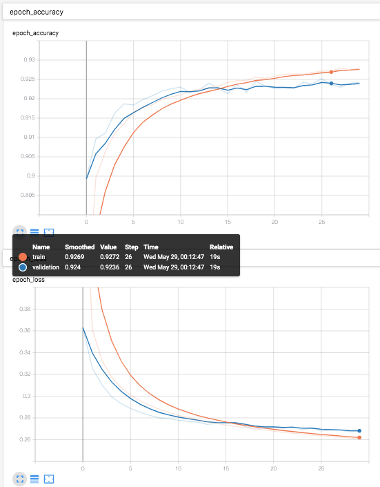
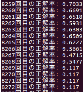
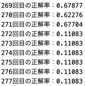
epoch数が8000回前半で学習がやや落ちていき、その後学習が出来なくなると行ったものです。
初めは学習回数が多いため、メモリがいっぱいになったことが原因であると考えましたが学習を分割して行なった際も同じ現象が起きたためメモリの問題でないことは分かりました。・分割した時の結果
次に考えたのは重みの更新が間違っているのではないかと考えました。
重みに正しい値が入らないことによって学習が出来なくなることを防ぐために重みの更新の部分のコードを以下のように訂正しました。・訂正前
tf.log(output)・訂正後
tf.log(tf.clip_by_value(output,1e-10,1.0))訂正前のものでは重みの値の範囲が指定されていないため重みの値に正しくない値が入ってしまうことがあります。
しかし、訂正後のものでは重みの値に範囲を指定しているため重みに正しくない値が入ることを防ぐことが出来ます。
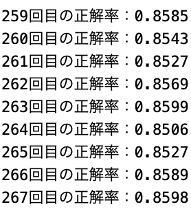
訂正後の結果は以下のようになった。
この結果の画像だけでは信憑性に欠けますが、重みの値を更新する際に範囲を指定することによって途中で学習が出来なくなることはなくなりました。
使っている教材としてオライリー・ジャパンのDeep Learningシリーズや初めてのtensorflowなどを使用しています。
- 投稿日:2019-05-24T11:43:12+09:00
RGB画像のみからの3次元人復元論文を読んでみた
RGB画像のみからの人の3D復元が今、熱い!?ということで論文を読んだので記事を書いてみます。
今まで3Dに触れたこともない素人なので間違っている箇所あれば編集リクエストなどお願いします。SMPLモデル
画像からの人の3D復元タスクはSMPLモデルと呼ばれるものを使うのが多いようです。
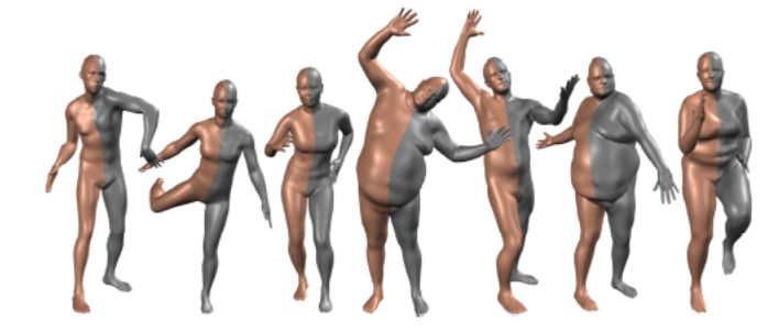
SMPLモデルとはA Skinned Multi-Person Linear Modelという論文で提案されたパラメータによる操作が可能な人体モデルです。(図は論文Fig1より)3Dモデルは一般的にとても複雑(mayaなどモデリングしている人すごい)なので、すべてのポリゴンを推定させようとすると困難です。そのため、あらかじめ低次元のパラメータで操作可能な人体モデルを作成することにより、3D推定をそのパラメータを推定させるタスクに置き換えることができます。
SMPLではheight,weight,(torso height)+(shoulder width),(chest breadth)+(neck height)などの10個の人のshapeを表す主成分特徴βと,72個のposeパラメータθを入力として1つの人体モデルが作ることができるようです。
βはSMPLモデルを作る際にデータセットの主成分分析を行い上位10個を用いているようです。
またposeパラメータの内訳は23個の関節のangleが関節1つにつき3つ、そして全体の向きを決定するglobal orientationが3つで3×23+3で72次元となります。
これにより,たとえばβのひとつ,左足の角度を連続的に変化させることにより簡単にポーズを変えることができます。
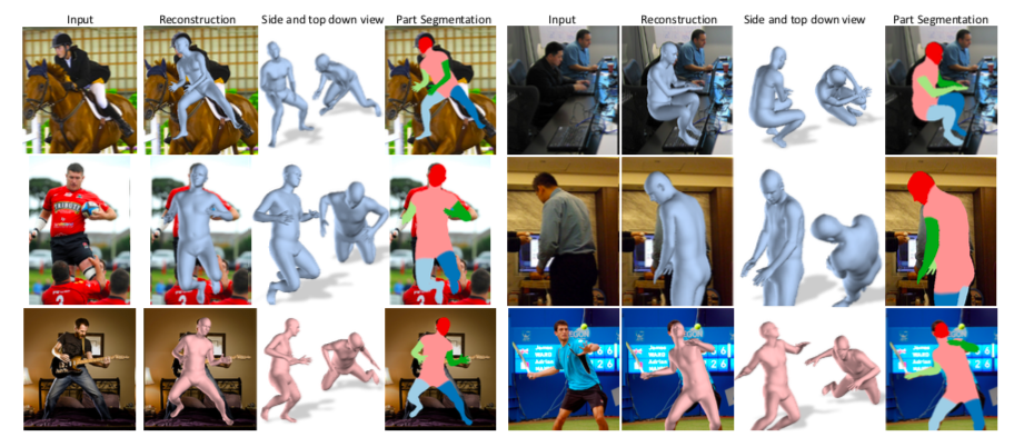
End-to-end Recovery of Human Shape and Pose
UCバークレーからのRGBからのSMPLモデルのパラメータ推定論文です。(Project page)
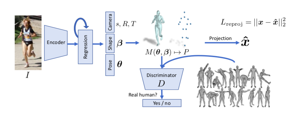
RGBからResnetベースでencodingしてSMPLモデルのβ、θを推定します。ただより正確な推定を行うために2次元平面へのreprojection LossとDiscriminator Lossを用いた学習をネットワークに追加しています。
reprojection Loss
3D復元の学習は学習データの作成がやはり難しくなります。またHuman3.6Mなどのデータセットは実験環境でデータが取られたこともあり、実際の煩雑な環境いわゆるin the wildな推定が困難とされてきました。そこでこの論文では2次元画像と3dモデルがunpairなデータセットでも学習できるようにSMPLモデルを2次元に投影し、2次元画像から取得した関節点座標とのlossをとるreporojection lossを提案しています。
θ、βを推定し、N=6980個の頂点をもつSMPLモデル
$M(\boldsymbol{\theta}, \boldsymbol{\beta}) \in \mathbb{R}^{3 \times \mathbb{N}}$
作成し,
keypoint頂点
$X(\boldsymbol{\theta}, \boldsymbol{\beta}) \in \mathbb{R}^{3 \times P}$
を得ます、
そしてさらにXをrotation,trasnlation,scaleのパラメータである
$R \in \mathbb{R}^{3 \times 3}$ ,$t \in \mathbb{R}^{2}$, $s \in \mathbb{R}$
を用いて2次元平面に投影します。
$\hat{\mathbf{x}}=s \Pi(R X(\boldsymbol{\theta}, \boldsymbol{\beta}))+t$
この$\hat{\mathbf{x}}$により、3Dモデルではなく2D正解データとのLossが計算できるようになります。よってencodeの段階ではθ、βだけではなくs,R,Tの推定も加えて85次元の$\Theta={\boldsymbol{\theta}, \boldsymbol{\beta}, R, t, s}$を推定します。
(θのglobal orientationがRのパラメータで取り込まれているのでθ=69次元になっている)
ただ、これを直接推定するのはかなり難しいらしく(特にR),iterative error feedbackと呼ばれる手法を用いています。iterative error feedbackは初期値$\Theta_{0}$を決め、従来の入力画像に$\Theta_{0}$を合わせたものを入力とします。ネットワークは$\Theta$ではなく目標値との残差$\Delta \Theta_{t}$を推定します。
そうして推定した$\Theta_{t+1}=\Theta_{t}+\Delta \Theta_{t}$を次の入力画像に加え推定を行うということにより、$\Delta \Theta_{t}$を最小化させ、段階的に推定精度を上げていくという手法のようです。参考論文 Human Pose Estimation with Iterative Error Feedback
また、3Dモデル正解データとの対応がとれる場合は勿論3Dモデル同士のLossが計算できて、頂点座標同士のLossと、β,θのパラメータLossを計算してreplojection lossに足すことができます。adversarial Loss
いままで3Dモデルを2Dに投影したときのlossを話してきましたが、勿論2Dだけでは3Dの正確な推定には無理があるのでadversarial Lossというものを追加します。GANで用いられるDiscriminatorと同じように、入力が生成されたものか、それともリアルデータかを判別するネットワークを追加することにより、より自然な復元を目指します。安定的な学習を行うためDはshape,poseごとに別々のDを用います。さらにはpose自体にも関節点ごとに最終層だけ異なるlayerをもつDを準備します。全部でK+2個のDiscriminatorです。(K個の関節θでK個、βで1個,pose全てを合わせたkinematic treeで1個) その分ネットワークは浅くすみ、学習は安定するようです。 ちなみにGANで起こりがちなmode collapseはDを騙すだけでなく、reprojection lossの制約もあるのであまりなかったと書いてます。
これまでの話しをまとめると損失関数は次のようになります.3Dlossは省略化ですL=\lambda\left(L_{\text { reproj }}+\mathbb{1} L_{3 \mathrm{D}}\right)+L_{\mathrm{adv}}L_{\text { reproj }}=\Sigma_{i}\left\|v_{i}\left(\mathbf{x}_{i}-\hat{\mathbf{x}}_{i}\right)\right\|_{1}L_{3 \mathrm{D}}=L_{3 \mathrm{D} \text { joints }}+L_{3 \mathrm{D} \text { smpl }}L_{\text { joints }}=\left\|\left(\mathbf{X}_{\mathbf{i}}-\hat{\mathbf{X}}_{\mathbf{i}}\right)\right\|_{2}^{2}L_{\mathrm{smpl}}=\left\|\left[\boldsymbol{\beta}_{i}, \boldsymbol{\theta}_{i}\right]-\left[\hat{\boldsymbol{\beta}}_{i}, \hat{\boldsymbol{\theta}}_{i}\right]\right\|_{2}^{2}\min L_{\mathrm{adv}}(E)=\sum_{i} \mathbb{E}_{\Theta \sim p_{E}}\left[\left(D_{i}(E(I))-1\right)^{2}\right]\min L\left(D_{i}\right)=\mathbb{E}_{\Theta \sim p_{\mathrm{data}}}\left[\left(D_{i}(\Theta)-1\right)^{2}\right]+\mathbb{E}_{\Theta \sim p_{E}}\left[D_{i}(E(I))^{2}\right]HMDやdensebodyなど主要論文をこれから追加しようと思ってます(いつになるかはわからない)
- 投稿日:2019-05-24T11:33:51+09:00
Bayesian Optimization for Hyperparameter Tuning
Source
- A Tutorial on Bayesian Optimization of Expensive Cost Functions, with Application to Active User Modeling and Hierarchical Reinforcement Learning
- Hyperparameter tuning in Cloud Machine Learning Engine using Bayesian Optimization
- Hyperparameter tuning on Google Cloud Platform is now faster and smarter
Introduction
Hyperparameters in neural networks are important; they define the network structure and affect model updates by controlling variables such as learning rates, optimization method and loss function. Therefore, it is imperative to find an efficient way of finding the optimal set of hyperparameters.
Quaint methods such as grid search are sluggish as they crawls through the entire search space and therefore end up wasting significant resource. By contrast, random search, which samples the search space randomly, ameliorates this effect and is widely used in practice. A drawback of random search, however, is that it doesn’t use information from prior experiments to select the next setting. This is particularly undesirable when the cost of running experiments is high and you want to make an educated decision on what experiment to run next.
Bayesian optimization is an extremely powerful technique when the mathematical form of the objective function is unknown or expensive to compute. The main idea behind it is to compute a posterior distribution (also called surrogate function) over prior (the objective function) based on the data (using the famous Bayes theorem), and then select good points to try with respect to this posterior distribution. If we can completely match the posterior with prior, then we can precisely determine the configuration of the hyperparameters which invokes the highest return.
Much of the efficiency stems from the ability of Bayesian optimization to incorporate prior belief about the problem to help direct the sampling, and to trade off exploration and exploitation of the search space.
Implementation
Goal
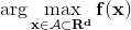
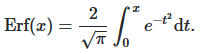
The main goal is to optimize a function $f(x)$ (which we will define as the performance of a function of hyperparameter values, e.g. model accuracy) over a compact set $A$ (the search space of the said hyperparameters), written mathematically as:
An example would be, if $f(x) = (1-x)e^x$, the maximum value $f(x) = 1$ will occur at $x = 0$ and so arg max is 0.
Bayes theorem states that the posterior probability of a model $M$ given evidence
(or data, or observations) $E$ is proportional to the likelihood of $E$ given $M$ multiplied by the prior probability of $M$:
Using the accumulated observation $D_{1:t}={x_{1:t},f(x_{1:t})}$, the prior is combined with the likelihood function $P(D_{1:t}|f)$, giving us:
Exploration-exploitation
Exploration: Pick a random place that may yield a good or bad result (variance is high).
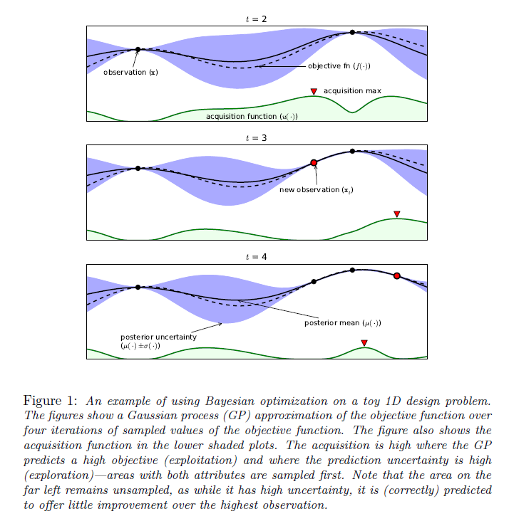
Exploitation: Pick a well acquainted place that have historically given fairly good result (mean is high). Although it may not be the best possible result available.Gaussian process (GP) is a distribution over functions specified by its mean function, $m$ and covariance function, $k$. It returns the mean and variance of a normal distribution.
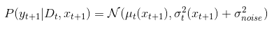
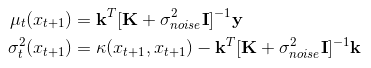
From the Gaussian process, we know that the predicted distribution (posterior) for the observed value at $x_{t+1}$ given the first $t$ observations, $D_t$ is:
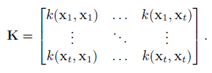
where
$y$ is the t-dimensional vector of observed values, and $K$ and $k$ are:
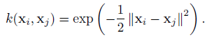
A very popular choice for $k$ is the squared exponential function:
The choice of covariance function $k$ is crucial, and the above squared exponential kernel might be slightly naive. It may be beneficial to introduce other parameters in order to control behaviours such as kernel width and smoothness.
Acquisition Function
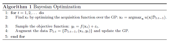
Rather than sampling randomly, Bayesian optimization uses acquisition function, which does automatic trade-off between exploration and exploitation. At each iteration, the acquisition function is maximized to determine where next to sample from the objective function. The objective is then sampled at the argmax of the acquisition function, and based on the return value from the objective function, the Gaussian process is updated and this process is repeated.
Bayesian optimization use evidence and prior knowledge to maximize the posterior at each step, so that each new evaluation decreases the distance between the true global maximum and the expected maximum.
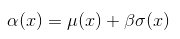
Upper confidence bound
Perhaps the simplest acquisition function looks at an optimistic value for the point. Given a parameter $\beta$, it assumes the value of the point will be $\beta$ standard deviations above the mean. Mathematically, it is
The equation would become $\alpha(x) = \mu(x) - \beta\sigma(x)$ for lower confidence bound if we were to find the minimum instead.
By varying $\beta$, we can encourage the algorithm to explore or exploit more. Note that the value for $\beta$ is left to the user.Probability of improvement
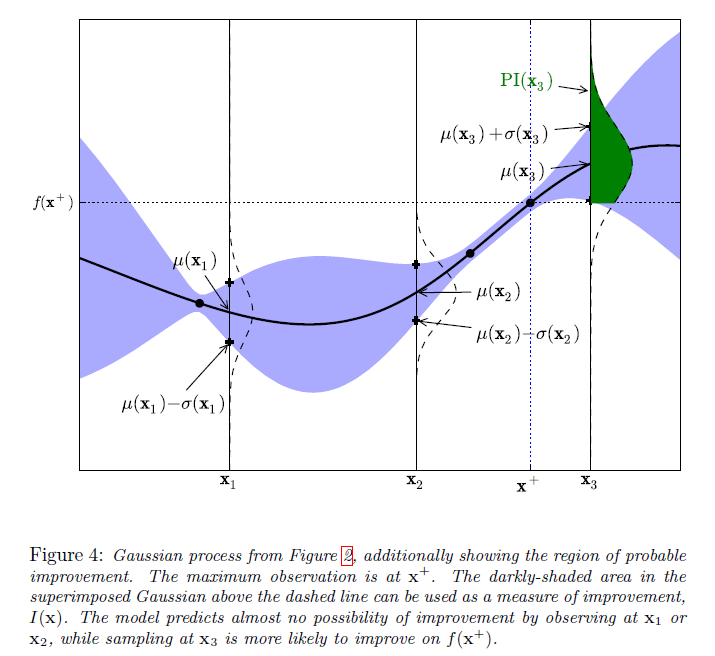
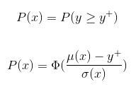
The main idea behind probability of improvement acquisition function is that we pick the next point based on the maximum probability of improvement (MPI) with respect to the current maximum.
Note that $y^+$ is the same as $f(x^+)$, $u(x)$ is the acquisition function, and $P(x)$ = $PI(x)$.In the above figure, the maximum observed value (so far), $y^+$ is at $x^+$. The area of the green shaded region gives the probability of improvement at $x_3$. The model predicts negligible possibility of improvement at $x_1$ or $x_2$. Whereas sampling at $x_3$ is likely to produce an improvement over $y^+$.
Where $\Phi$ is normal cumulative distribution function (the probability that a random variable $X$ will take a value less than or equal to $x$).Expected Improvement
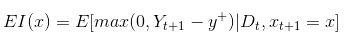
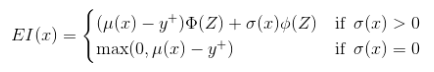
The algorithm which Google's Cloud ML Engine uses for acquisition function is called Expected Improvement. It measures the expected increase in the maximum objective value seen over all experiments, given the next point we pick. In contrast, MPI only takes into account the probability of improvement and not the magnitude of improvement for the next point. Mathematically, as proposed by Mockus, it is
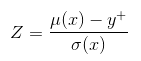
where the expectation is taken over $Y_{t+1}$ which is distributed as the posterior objective value at $x_{t+1}$ In other words, if the objective function were drawn from our posterior distribution, then $EI(x)$ measures the expected increase in the best objective we have found during entire tuning run if we select $x$ and then stop.When using a Gaussian process we can obtain the following analytical expression for EI
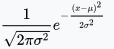
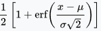
Where $Z$ has the expression denoted below and $\phi$ and $\Phi$ denote the probability density function (PDF) and cumulative distribution function (CDF) of the standard normal distribution function.
$\phi$ =
$\Phi$ =
Bayesian Optimization Algorithm
Result
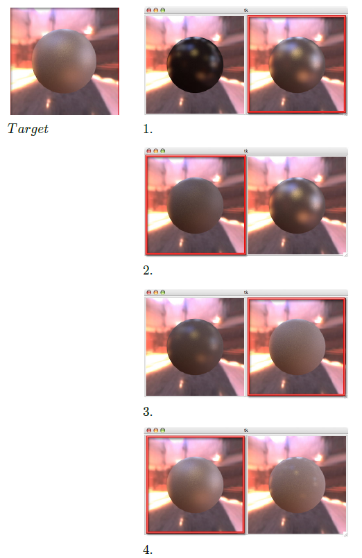
Interactive Bayesian optimization for material design
In the above figure, the user would select from the provided two images, one that most resembles the target image at each iteration.
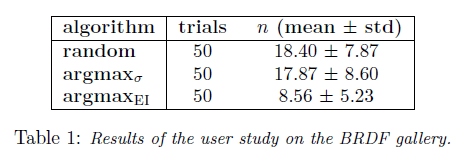
It can be seen that $argmax_{EI}$ requires conspicuously fewer iterations in order to derive the correct material parameters.Conclusion
Searching for hyperparameters can be made more efficiently through the usage of Bayesian Optimization. There are actually further under the hood features implemented by Google for their AI Platform hyperparameter tuning service that further improves the quality of life during parameter searching. Options such as early stopping, where the system stops parameter searching if it determines a better configuration does not exist, and learning from previously visited parameter set in order to speed up the algorithm when expanding on the parameter space.
There are of course other issues, such as handling the trade-off between exploration and exploitation in the acquisition function. Or the fact that the acquisition is only looking one-step ahead (although it should be able to implement multi-step through recursion). There may have been other advancements made in recent years that will require further investigation.

- 投稿日:2019-05-24T10:26:15+09:00
【画像生成】AutoencoderとVAEと。。。遊んでみた♬AEとその潜在空間は???
昨夜のお約束の「DLの記憶」について書く準備として、AEと潜在空間について記事にしておこうと思います。
※DLの記憶はこの次の記事にしますやったこと
・通常のAEでVAEと同様な絵を作成する
・潜在空間内の画像生成
・潜在空間を移動させて画像生成する・通常のAEでVAEと同様な絵を作成する
通常のAEを以下のように改変してVAEと同じようなことができるか試してみました。
それは、どうしてもあのLatent_dimのところでGauss関数に押し込む必要性が合点できないからです。
すなわち、あの関数はどんなものでもよく(たぶん、BackPropagationできる程度に滑らかなら)、全体のAEとしての機能は変わらないだろうと考察されるからです。逆に言えば、自然に発生する分布(関数と呼んでいいかは別として)を利用しても同じように制御できる可能性があるということで、やってみました。
これはよく説明に「AEは入力を再現するだけ、VAEは自由に画像生成することができる。」すなわち「AEは自由に画像生成できない」というのは誤解だということが元々のモチベーションですコードは以下のとおりです。
変更点は、z_log_varを止めて、z_meanだけにしようということだけです。
この選択により、sampling関数は不要になります。
※分布は野となれ山となれということになります
すなわち、つなぎの部分が全結合になっていますが、通常のAEです。inputs = Input(shape=input_shape, name='encoder_input') x = Conv2D(32, (3, 3), activation='relu', strides=2, padding='same')(inputs) x = Conv2D(64, (3, 3), activation='relu', strides=2, padding='same')(x) shape = K.int_shape(x) print("shape[1], shape[2], shape[3]",shape[1], shape[2], shape[3]) x = Flatten()(x) z_mean = Dense(latent_dim, name='z_mean')(x) # instantiate encoder model encoder = Model(inputs, z_mean, name='encoder') encoder.summary()decoderも通常のまんまです。
# build decoder model
latent_inputs = Input(shape=(latent_dim,), name='z_sampling')
x = Dense(shape[1] * shape[2] * shape[3], activation='relu')(latent_inputs)
x = Reshape((shape[1], shape[2], shape[3]))(x)
x = Conv2DTranspose(64, (3, 3), activation='relu', strides=2, padding='same')(x)
x = Conv2DTranspose(32, (3, 3), activation='relu', strides=2, padding='same')(x)
outputs = Conv2DTranspose(1, (3, 3), activation='sigmoid', padding='same')(x)
# instantiate decoder model
decoder = Model(latent_inputs, outputs, name='decoder')
decoder.summary()
# instantiate VAE model
outputs = decoder(encoder(inputs))
vae = Model(inputs, outputs, name='vae_mlp')
異なるのは、この後に描画関数(おまけに掲載)をVAEと同じものを使います。
結果として以下のような図が得られます。
以下で示す図も含め、これらの図はほぼsampling関数を利用したものと変わりません。
・潜在空間内の画像生成
画像生成の制御もある意味簡単にできることが分かります。
以下は、おまけに掲載したコードで生成した潜在空間内で生成された画像です。
この絵を見ると、母関数としてガウス分布を仮定しなくとも、画像はバラバラに生成されているわけではなく、分類・適度に分散されながら生成されていることが分かります。
※この部分が実はあとあと面白い解釈ができるのですが、次回の議論とします
・潜在空間を移動させて画像生成する
そして、上記の潜在空間内を連続的に移動しながら画像生成します。
下記のように問題なく画像生成できます。
つまり、上に示した画像の潜在空間内の分布はガウス分布などの母関数を仮定しなくとも、画像生成は連続する変化となっており、途中の変化がなめらかになっているところがミソです。
以下のパラメータ変換で、潜在空間内の点を移動させながらdecoderで画像生成しています。
【参考】以下を参考にしています
Variational Autoencoder徹底解説z : s*z_0 + (1-t)*z_1def plot_results2(models, data, batch_size=128, model_name="vae_mnist"): z0=np.array([0.4,-2.3]) z1=np.array([0.4,2.7]) for t in range(50): s=t/50 z_sample=np.array([s*z0+(1-s)*z1]) x_decoded = decoder.predict(z_sample) plt.imshow(x_decoded.reshape(28, 28)) plt.title("z_sample="+str(z_sample)) plt.savefig('./mnist1000/z_sample_t{}'.format(t)) plt.pause(0.1) plt.close()※上記は50分割にしていますが、これはアップの都合でそうしているだけで、性能的には10倍くらいにしても問題なく動きます
以下のように円上を360度動かして、小さいサイズ(2.5MB位)にしたけど、やはりアップできないので、出来るようになったらアップすることとします。
円上を動かすコードは以下のとおりdef plot_results2(models, data, batch_size=128, model_name="vae_mnist"): for t in range(360): s=t/360 z_sample=np.array([[2*np.cos(2*s*np.pi),2*np.sin(2*s*np.pi)]]) x_decoded = decoder.predict(z_sample) plt.imshow(x_decoded.reshape(28, 28)) plt.title("z_sample="+str(t)) plt.savefig('./mnist1000/360/z_sample_t{}'.format(t)) plt.pause(0.01) plt.close()【参考】z0=np.array([0.4,-2.3])などとしている理由は以下の参考のとおりです
・Why do I get TypeError: can't multiply sequence by non-int of type 'float'?まとめ
・AEで潜在空間のパラメータを動かして画像生成できた
・潜在空間内でパラメータを自由に動かしたとき滑らかに画像生成できることが分かった・潜在空間内での画像生成と元の学習データの関係についてはDLの記憶とともに次回記事にします
おまけ
def plot_results(models,
                 data,
                 batch_size=32,
                 model_name="vae_mnist"):
    """Plots labels and MNIST digits as function of 2-dim latent vector
    # Arguments
        models (tuple): encoder and decoder models
        data (tuple): test data and label
        batch_size (int): prediction batch size
        model_name (string): which model is using this function
    """
    encoder, decoder = models
    x_test, y_test = data
    os.makedirs(model_name, exist_ok=True)

    filename1 = "./mnist1000/vae_mean100L2_3"
    # display a 2D plot of the digit classes in the latent space
    z_mean = encoder.predict(x_test, batch_size=batch_size)
    plt.figure(figsize=(12, 10))
    plt.scatter(z_mean[:, 0], z_mean[:, 1], c=y_test)
    plt.colorbar()
    plt.xlabel("z[0]")
    plt.ylabel("z[1]")
    plt.savefig(filename1+"z0z1.png")
    plt.pause(1)
    plt.close()

    filename2 = "./mnist1000/digits_over_latent100L2_3"
    # display a 30x30 2D manifold of digits
    n = 30
    digit_size = 28
    figure = np.zeros((digit_size * n, digit_size * n))
    # linearly spaced coordinates corresponding to the 2D plot
    # of digit classes in the latent space
    grid_x = np.linspace(-4, 4, n)
    grid_y = np.linspace(-4, 4, n)[::-1]
    for i, yi in enumerate(grid_y):
        for j, xi in enumerate(grid_x):
            z_sample = np.array([[xi, yi]])
            x_decoded = decoder.predict(z_sample)
            digit = x_decoded[0].reshape(digit_size, digit_size)
            figure[i * digit_size: (i + 1) * digit_size,
                   j * digit_size: (j + 1) * digit_size] = digit
    plt.figure(figsize=(10, 10))
    start_range = digit_size // 2
    end_range = n * digit_size + start_range + 1
    pixel_range = np.arange(start_range, end_range, digit_size)
    sample_range_x = np.round(grid_x, 1)
    sample_range_y = np.round(grid_y, 1)
    plt.xticks(pixel_range, sample_range_x)
    plt.yticks(pixel_range, sample_range_y)
    plt.xlabel("z[0]")
    plt.ylabel("z[1]")
    plt.imshow(figure, cmap='Greys_r')
    plt.savefig(filename2+".png")
    plt.pause(1)
    plt.close()


![z_sample_t_NoSamplingz0=[0.4,-2.3]z7=[0.4,2.7].gif](https://qiita-image-store.s3.ap-northeast-1.amazonaws.com/0/233744/064b5a51-2e0d-4c46-cdfb-0a4d61cf39d9.gif)
- 投稿日:2019-05-24T01:27:10+09:00
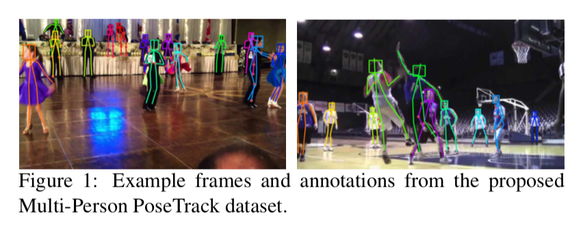
論文まとめ:PoseTrack: Joint Multi-Person Pose Estimation and Tracking
はじめに
CVPR2017から以下の論文
[1] U. Iqbal, et. al. "PoseTrack: Joint Multi-Person Pose Estimation and Tracking"
のまとめ同じ著者らの似た論文で CVPR2018に "PoseTrack: A Benchmark for Human Pose Estimation and Tracking"というものがあるが、こちらは名前の通りbenchmarkやsurveyに関する論文。
著者らの公式githubコード。
https://github.com/iqbalu/PoseTrack-CVPR2017その他、同じCVPR2017でacceptされた有名論文で
[2] E. Insafutdinov, et. al. "ArtTrack: Articulated Multi-person Tracking in the Wild"
というものがある。以下、主にロジック部分のみまとめ。
概要
- ビデオ映像の中の複数人に対して骨格の推定とtrackingを行うモデル
- 関節の候補位置を推定させ、それを時空間のグラフ問題として整数線形計画法で解く
以下の[1]Figure1のようにビデオ映像に対して骨格を推定する
モデル
モデルの全体像
以下の[1] Figure2で説明すると
まずはじめに、上段のようにビデオ映像の各フレームに対して関節(カラーの丸)を推定する。
次に中段のように、同じフレーム内でのある関節と別の関節との対応づけ(青線)、及びフレーム間に渡り同じ関節での対応づけ(赤線と黄色線)を行う。ここでは整数線形計画法を用いて最適化問題を解く。
最後に下段のようにそれらから各個人の骨格を推定する。
時空間グラフの構築
複数のフレームからなるビデオ $\mathcal{F}$ があり、各フレーム $f$ には任意の人が写っている。ビデオにおける関節候補 $D$ は、各フレーム $f$ における関節の候補 $D_f$ の全フレームにわたる集合。
D = \{D_f \}_{f\in\mathcal{F}}また $\bf{x}\rm^f_d \in \mathbb{R}^2$ はフレーム $f$におけるある関節 $d \in D$ における座標。この $d$ はいずれかの関節タイプ $j \in \mathcal{J} = { 1, \cdots ,J }$ に属する。
本論文の課題である「多人数骨格トラッキング」は以下の時空間グラフ $G$
G = (D,E)を推定する問題である。
ここで $E$ はedgesであり、任意の関節と関節とを結ぶ。これには2種類あって、同じフレームで空間的に結ぶ $E_s$ (例えばAさんの右肩とBさんの右肘)と、時間軸にわたって同じ関節を結ぶ $E_t$ (例えばフレーム3におけるAさんの右肩とフレーム4におけるAさんの右肩)がある。
つまり $E_s$ は
E_s = \cup_{f \in \mathcal{F}} E^f_s \ and \ E^f_s \{ (d,d'):d \neq d' \land d,d' \in D_f \}で、$E_t$ は
E_t = \{ (d,d'):j = j' \land d \in D_f ,d' \in D_{f'} \land 1 \leq |f-f'| \leq \tau \land f, f' \in \mathcal{F} \}である。
$1 \leq |f-f'| \leq \tau$ という制約があるので一定間隔以内のフレーム同士のみで考えている。隣同士のフレームのみでないのは、オクルージョンに対応するため。
グラフ分割
時空間グラフ $G$ には実際に関節ではない $D$ (以下nodesともいう)と、関係ないつながり(edges)・・・例えば同じフレーム内のAさんの右肩とBさんの左肩、あるいは異なるフレーム間でのAさんの右手とAさんの右足、など・・・が多数ある。このグラフを分割したい。
変数等の定義
そこで以下のバイナリー値を導入する。
\begin{eqnarray*}
v&\in& \{ 0,1 \}^{|D|}\\
s&\in& \{ 0,1 \}^{|E_s|}\\
t&\in& \{ 0,1 \}^{|E_t|}\\
\end{eqnarray*}
$v=0$ なら検出した関節候補は関節でないので削除する。
s_{(d_f, d'_f)}=0また
t_{(d_f, d'_{f'})}=0なら異なるフレーム間の時間的edgeである $(d_f, d'_{f'})$ は削除される。
目的関数
このグラフ分割は以下のコスト関数を最小化することにより達成する。
\newcommand{\argmin}{\mathop{\rm arg~min}\limits}
\begin{eqnarray*}
&&\argmin_{v,s,t} (<v,\phi >+<s,\psi_s >+<t,\psi_t>) \\
&&<v,\phi> = \sum_{d \in D} v_d \phi(d) \\
&&<s,\psi_s > = \sum_{(d_f,d'_f) \in E_s} s_{(d_f,d'_f)} \psi_s (d_f, d'_f) \\
&&<s,\psi_t > = \sum_{(d_f,d'_{f'}) \in E_t} t_{(d_f,d'_{f'})} \psi_t (d_f, d'_{f'})
\end{eqnarray*}
ここで $\phi$ 、 $\psi_s$ 、 $\psi_t$ はそれぞれ
\begin{eqnarray*}
&&\phi(d) = \log \frac{1-p_d}{p_d} \\
&&\psi_s(d_f,d'_f) = \log \frac{1-p^s_{(d_f,d'_f)}}{p^s_{(d_f,d'_f)}} \\
&&\psi_t(d_f,d'_{f'}) = \log \frac{1-p^t_{(d_f,d'_{f'})}}{p^t_{(d_f,d'_{f'})}} \\
\end{eqnarray*}
$p_d \in (0,1)$ は予測した関節 $d$ の確率。$p^s$ はフレーム $f$ における $d$ と $d'$ の結合に関する確率。$p^t$ はフレーム $f$ における $d$ と フレーム $f'$ における $d'$ の結合に関する確率。
制約式
これらを整数線形計画法で解くが、そのときの制約は以下。
まず制約の1種類目。
s_{(d_f, d'_f)} \leq v_{d_f} \land s_{(d_f, d'_f)} \leq v_{{d'}_f} \ \ \  \forall (d_f,d'_f) \in E_s \\
t_{(d_f, d'_{f'})} \leq v_{d_f} \land t_{(d_f, d'_{f'})} \leq v_{{d'}_{f'}} \ \ \  \forall (d_f,d'_{f'}) \in E_t
上の式は同じフレーム $f$ において関節 $d_f$ と $d'_{f}$ がともに有効な時のみ両者の空間的 edge は有効とするもの。
下の式は異なるフレーム間の関節 $d_f$ と $d_{f'}$ 間において、それらが有効な時のみ両者の時間的 edge を有効とするもの。
次に制約の2種類目。
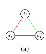
s_{(d_f, d'_f)} + s_{(d'_f, d''_f)} - 1 \leq  s_{(d_f, d''_f)}\\
\forall (d_f, d'_f), (d'_f, d''_f) \in E_s
つまり以下の図のように
同じフレーム $f$ 内の3つの node に関して、2つの edge が有効なら、残りの1つの edge も有効とするもの。
同様に異なるフレーム間3つの node に関して、2つの edgeが有効なら、残りの1つの edge も有効とする。
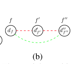
t_{(d_f, d'_{f'})} + t_{(d'_{f'}, d''_{f''})} - 1 \leq  t_{(d_f, d''_{f''})}\\
\forall (d_f, d'_{f'}), (d'_{f'}, d''_{f''}) \in E_t
図で書くとこう。
次の制約式は骨格が一定と想定するもの。
t_{(d_f, d'_{f'})} + t_{(d_{f}, d''_{f'})} - 1 \leq  s_{(d'_{f'}, d''_{f'})}\\
t_{(d_f, d'_{f'})} + s_{(d'_{f'}, d''_{f'})} - 1 \leq  t_{(d_{f}, d''_{f'})}\\
\forall (d_f, d'_{f'}), (d_{f}, d''_{f'}) \in E_t
最後の制約式は異なるフレーム間の4つの node に関するもの。
t_{(d_f, d'_{f'})} + t_{(d''_{f}, d'''_{f'})} + s_{(d_{f}, d''_{f})} - 2 \leq  s_{(d'_{f'}, d'''_{f'})}\\
t_{(d_f, d'_{f'})} + t_{(d''_{f}, d'''_{f'})} + s_{(d'_{f'}, d'''_{f'})} - 2 \leq  s_{(d_{f}, d''_{f})}\\
\forall (d_f, d'_{f'}), (d''_{f}, d'''_{f'}) \in E_t
んー、最後はややこしいな。

- 投稿日:2019-05-24T00:26:55+09:00
グラフニューラルネットワークの資料リンク
グラフニューラルネットワークの勉強会で使った資料です
ハンズオン資料
とりあえず動かしてみる
DGL at a Glance — DGL 0.2 documentationグラフメッセージ伝搬でみるページランク
PageRank with DGL Message Passing — DGL 0.2 documentationモデルのチュートリアル
Model overview — DGL 0.2 documentation
- ローカルで環境構築できなかった場合、こちらのgoogle colabを試してみる手もある:
1_first.ipynb - Google ドライブ面白そうな応用研究
- Pinterestのリコメンドシステム(A/BテストでKPIが30%改善): PinSage: A new graph convolutional neural network for web-scale recommender systems、PinSage: A new graph convolutional neural network for web-scale recommender systems
参考資料
- 論文集(Survey papersの最初の三本がいい):GitHub - thunlp/GNNPapers: Must-read papers on graph neural networks (GNN)
- Yann LeCunの講演:YouTube
- 著者による原論文のブログ解説記事:Graph Convolutional Networks | Thomas Kipf | PhD Student @ University of Amsterdam
その他のリソース
- ナレッジグラフ:Wikidata
- ナレッジグラフの埋め込み:GitHub - facebookresearch/PyTorch-BigGraph: Software used for generating embeddings from large-scale graph-structured data.
- ポアンカレ埋め込みの実装:GitHub - facebookresearch/poincare-embeddings: PyTorch implementation of the NIPS-17 paper "Poincaré Embeddings for Learning Hierarchical Representations"
dgl以外のライブラリ
chainerの化学用ライブラリ:
GitHub - pfnet-research/chainer-chemistry: Chainer Chemistry: A Library for Deep Learning in Biology and Chemistry, 化学、生物学分野のための深層学習ライブラリChainer Chemistry公開 | Preferred ResearchPytorch用の化学用ライブラリ
GitHub - deepchem/deepchem: Democratizing Deep-Learning for Drug Discovery, Quantum Chemistry, Materials Science and Biologypytorch geometric(dglの競合?ビルドはcuda10の方がすんなりいく、と思う)
GitHub - rusty1s/pytorch_geometric: Geometric Deep Learning Extension Library for PyTorchDeepMind提供、趣が少し違うが、元論文の最初の方はなぜグラフなのかについて説明してあって、一読の価値がある:GitHub - deepmind/graph_nets: Build Graph Nets in Tensorflow