- 投稿日:2019-05-23T23:53:40+09:00
Raspi 3 + USB Accelerator で画像分類&物体検出
Raspberry PiとUSB Acceleratorを使って
画像分類と物体検出をしてみました。行ったのは、公式のスタートガイドです。
環境
- Raspberry Pi 3 Model B+
- ubuntu mate
Raspberry Pi のセットアップ
Edge TPU runtimeとPythonライブラリをインストールします
$ cd ~/
$ wget https://dl.google.com/coral/edgetpu_api/edgetpu_api_latest.tar.gz -O edgetpu_api.tar.gz --trust-server-names
$ tar xzf edgetpu_api.tar.gz
$ cd edgetpu_api
$ bash ./install.sh
install.shを実行するとWould you like to enable the maximum operating frequency?と聞かれます。
最大でパフォーマンスでUSB Acceleratorを使うと、USB Acceleratorがとても熱くなり、やけどするかもしれないので、
最大パフォーマンスが必要かどうか分からないならNにしろ、とのことです。
この設定は後からでも変えられるそうです。デモの実行
画像分類
サンプルデータをダウンロード
cd ~/Downloads/

wget https://dl.google.com/coral/canned_models/mobilenet_v2_1.0_224_inat_bird_quant_edgetpu.tflite \
https://dl.google.com/coral/canned_models/inat_bird_labels.txt \
https://coral.withgoogle.com/static/images/parrot.jpg
ラズパイを日本語で設定している方は
Downloadsというディレクトリがないと思います。
その場合は、適当なディレクトリでよいです。デモの実行
$ cd /usr/local/lib/python3.5/dist-packages/edgetpu/demo

$ python3 classify_image.py \
--model ~/Downloads/mobilenet_v2_1.0_224_inat_bird_quant_edgetpu.tflite \
--label ~/Downloads/inat_bird_labels.txt \
--image ~/Downloads/parrot.jpg
modellabelimageのファイルパスは、ダウンロード先に合わせて変更してください。
実行に成功すると、以下のような出力がされます。Ara macao (Scarlet Macaw) Score : 0.746094物体検出
サンプルデータをダウンロード
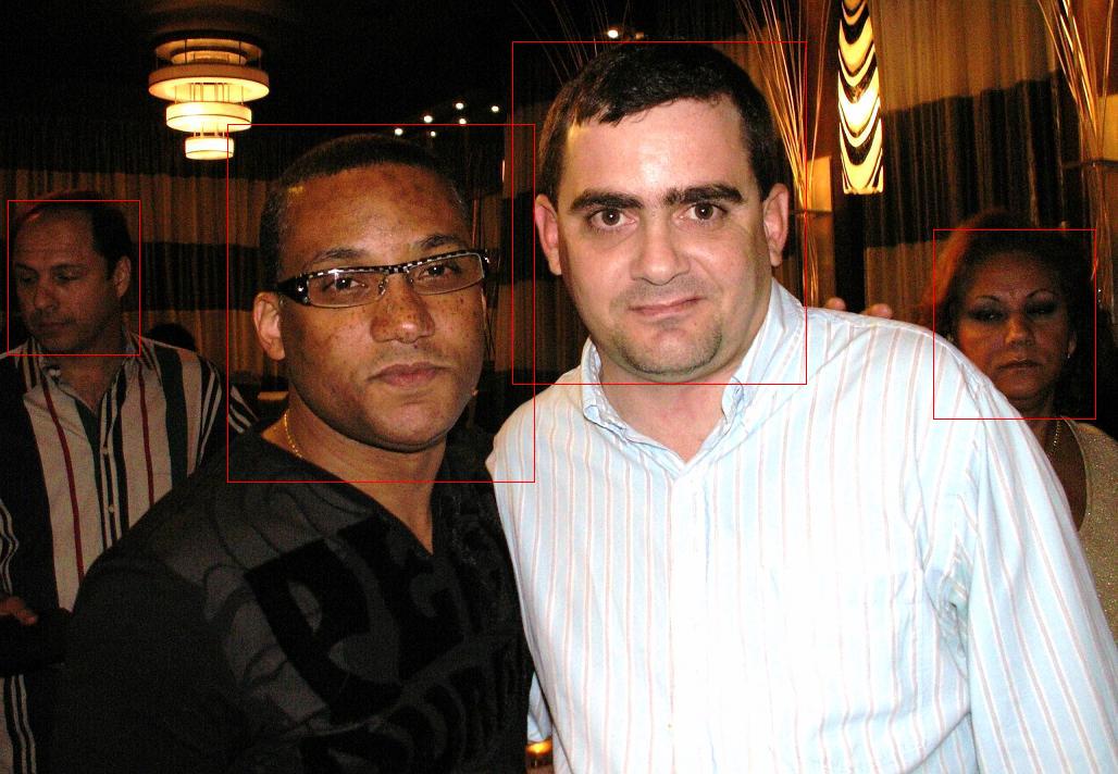
cd ~/Downloads/

wget https://dl.google.com/coral/canned_models/mobilenet_ssd_v2_face_quant_postprocess_edgetpu.tflite \
 https://coral.withgoogle.com/static/images/face.jpg
デモの実行
$ cd /usr/local/lib/python3.5/dist-packages/edgetpu/demo

$ python3 classify_image.py \
--model ~/Downloads/mobilenet_v2_1.0_224_inat_bird_quant_edgetpu.tflite \
--label ~/Downloads/inat_bird_labels.txt \
--image ~/Downloads/parrot.jpg
もし実行エラーとなって
No such file or directory: 'feh'というメッセージが表示されたら
sudo apt-get install fehとしてから、再実行してください。以下のような表示がされば成功です。
-----------------------------------------
score =  0.996094
box =  [471.33392310142517, 38.03488787482766, 741.695974111557, 353.5309683683231]
-----------------------------------------
score =  0.996094
box =  [209.30670201778412, 114.17187392981344, 491.6300288438797, 443.6261138225572]
-----------------------------------------
score =  0.832031
box =  [7.304725393652916, 184.98179422784176, 128.21268820762634, 326.07404544882104]
-----------------------------------------
score =  0.5
box =  [858.2628228664398, 211.6830582424526, 1007.3986599445343, 385.80091726725993]
リアルタイム画像分類 & 物体検出
ラズパイ用カメラやUSBカメラから取得した画像に対して、リアルタイムで画像分類&物体検出ができるデモもあります。
デモ用プログラムの取得
$ git clone https://github.com/google-coral/examples-camera.gitサンプルデータをダウンロード
cd ~/Downloads/

# 物体分類用
wget https://dl.google.com/coral/canned_models/mobilenet_v2_1.0_224_quant_edgetpu.tflite \
 https://dl.google.com/coral/canned_models/imagenet_labels.txt

# 物体検出用
wget https://dl.google.com/coral/canned_models/mobilenet_ssd_v2_coco_quant_postprocess_edgetpu.tflite \
 https://dl.google.com/coral/canned_models/coco_labels.txt
ラズパイカメラでの画像分類
事前にカメラが使えるよう
pip3 install picameraとraspi-configでカメラを有効にしてください。$ cd examples-camera/raspicam $ python3 classify_capture.py --model ~/Downloads/mobilenet_v2_1.0_224_quant_edgetpu.tflite --labels ~/Downloads/imagenet_labels.txtウィンドウに画像が表示され、画面の上部に分類結果などが表示されれば成功です。
USBカメラによる画像分類
実行前に、
gstreamなどのインストールをする必要があります。$ cd examples-camera/gstreamer $ sh install_requirements.sh実行
$ cd examples-camera/gstreamer
$ python3 classify_capture.py --model ~/Downloads/mobilenet_v2_1.0_224_quant_edgetpu.tflite --labels ~/Downloads/imagenet_labels.txt
こちらもウィンドウに画像が表示され、画面の上部に分類結果などが表示されれば成功です。
USBカメラによる物体検出
$ cd examples-camera/gstreamer
$ python3 classify_capture.py --model ~/Downloads/mobilenet_ssd_v2_coco_quant_postprocess_edgetpu.tflite --labels ~/Downloads/coco_labels.txt
ウィンドウに画像が表示され、物体検出の結果であるバウンディングボックスなどが表示されれば成功です。
こちらの環境では、たまに飛ぶことがあるものの、約5fpsくらいで動作しました。他のサンプルデータ
ここのREADMEの一番下に、サンプルデータの一覧が記載してあります。
- 投稿日:2019-05-23T17:21:22+09:00
対決!RTX 2080Ti SLI vs Google Colab TPU ~PyTorch編~
RTX 2080Tiを2枚使って頑張ってGPUの訓練を高速化する記事の続きです。TensorFlowでは複数GPU時に訓練が高速化しないという現象がありましたが、PyTorchを使うとRTX 2080Tiでもちゃんと高速化できることを確認できました。これにより、2GPU時はTensorFlowよりも大幅に高速化できることがわかりました。
前回までの記事
ハードウェアスペック
- GPU : RTX 2080Ti 11GB Manli製×2 SLI構成
- CPU : Core i9-9900K
- メモリ : DDR4-2666 64GB
- CUDA : 10.0
- cuDNN : 7.5.1
- PyTorch : 1.1.0
- Torchvision : 0.2.2
前回と同じです。「ELSA GPU Monitor」を使って、GPUのロードや消費電力をモニタリングします(5秒ごとCSV出力)。
結果
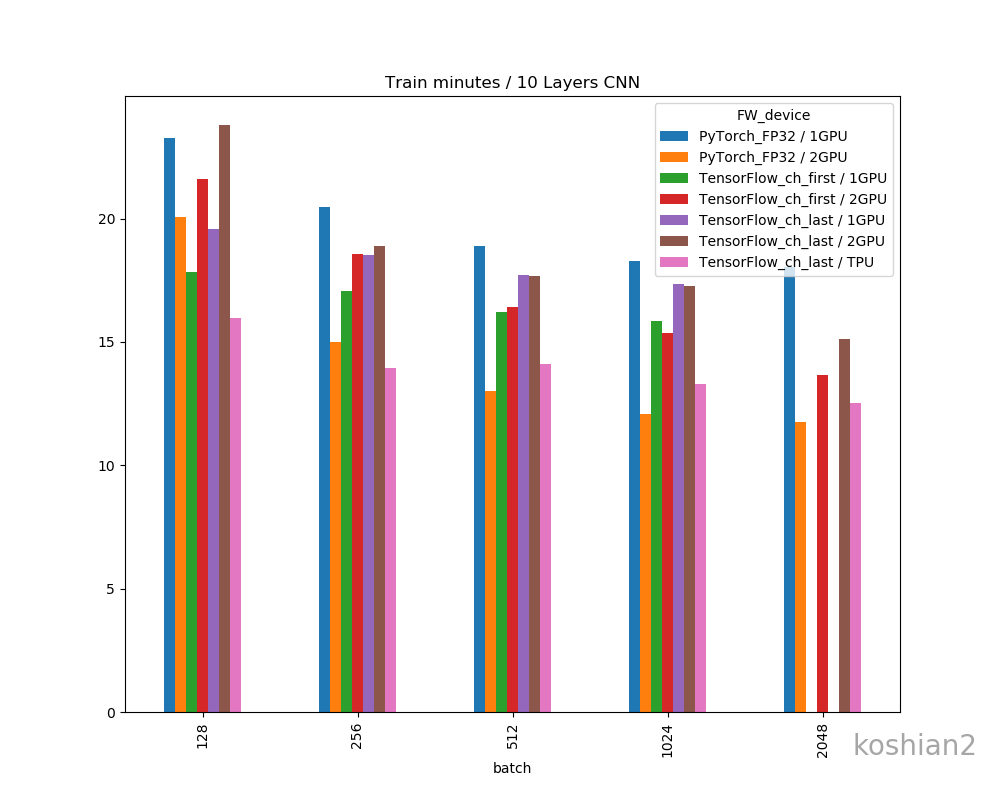
10層CNN
10層CNNの詳細は初回の記事を参照してください。縦軸に訓練時間、横軸にバッチサイズを取ったものです。
「TensorFlow_ch_first」はこちらで書いたTensorFlowかつchannels_firstとしたケースです。「TensorFlow_ch_last」はchannels_lastのケースで、TensorFlow/Kerasのデフォルトの設定はchannels_lastになります。
「1GPU, 2GPU」はRTX2080Tiの数で、2GPUの場合は、TensorFlowは
multi_gpu_modelを使い、データパラレルとして並列化させています。PyTorchの場合は、if use_device == "multigpu": model = torch.nn.DataParallel(model)このように同じくデータパラレルで並列化させています。大きいバッチでデータのないところは、OOMになってしまうため測っていない場所です。
このグラフから以下のことがわかります。
- 小さいCNNかつ1GPUでは、必ずしもPyTorchが最速とは限らない。むしろTensorFlow、特にchannels_firstにしたTensorFlowのほうが速いことがある。
- TensorFlowとPyTorchの差は、小さいCNNではバッチサイズを大きくすると縮まっていく。
- ただし、PyTorchでは2GPUにしたときは明らかにTensorFlowよりも速くなる。バッチサイズ512以降では、Colab TPUよりもFP32で既に速い。
- PyTorchのほうが大きいバッチサイズを出しやすい。TensorFlowの場合は、1GPUではバッチサイズが2048のケースがOOMで訓練できなかったが、PyTorchの場合は1GPUでバッチサイズ2048を訓練できる。
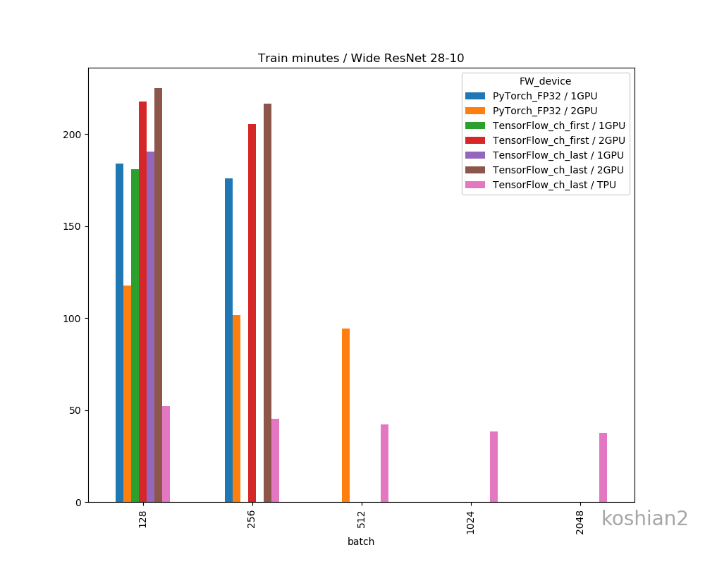
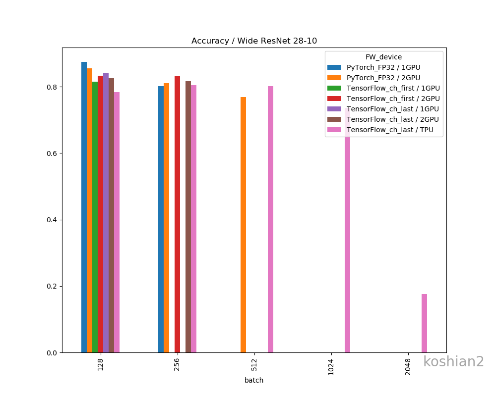
Wide ResNet 28-10
こちらはWide ResNet 28-10の訓練時間を比較したものです。
- 大きいCNNかつ1GPUでは、PyTorchとTensorFlowの訓練時間の差はほとんどない。特にTensorFlowでChannels firstにすればPyTorchかそれ以上の速さは出せる。
- しかし、複数GPUになると、明らかにPyTorchのほうが速くなる。TensorFlowのGPU並列化が何かおかしい。
- ただし、WRNのような大きなCNNのでは、PyTorch+2GPU+FP32ではまだColab TPUに勝てなかった
- PyTorchの場合、TensorFlowのできなかった1GPUでのバッチサイズ256、2GPUのバッチサイズ512を訓練することができた。なぜかPyTorchのほうが訓練できるバッチサイズが大きい。
PyTorch個別の結果
今回やったPyTorchだけの結果を表します
1GPU・10層CNN
バッチ 1エポック[s] 2~中央値[s] 訓練時間 精度 128 15.86 13.90 0:23:15 0.8915 256 12.72 12.29 0:20:28 0.8900 512 13.60 11.33 0:18:53 0.8837 1024 16.52 10.93 0:18:17 0.8860 2048 15.50 10.80 0:18:03 0.8639 1GPU・WRN
バッチ 1エポック[s] 2~中央値[s] 訓練時間 精度 128 111.89 110.42 3:03:57 0.8743 256 105.71 105.47 2:55:48 0.8011 2GPU・10層CNN
バッチ 1エポック[s] 2~中央値[s] 訓練時間 精度 128 16.07 11.92 0:20:04 0.8896 256 8.96 9.00 0:15:00 0.8912 512 8.74 7.80 0:13:01 0.8816 1024 9.52 7.24 0:12:05 0.8814 2048 8.34 7.05 0:11:45 0.8688 2GPU・WRN
バッチ 1エポック[s] 2~中央値[s] 訓練時間 精度 128 72.75 70.58 1:57:38 0.8559 256 58.43 60.83 1:41:22 0.8109 512 59.01 56.49 1:34:14 0.7695 精度比較
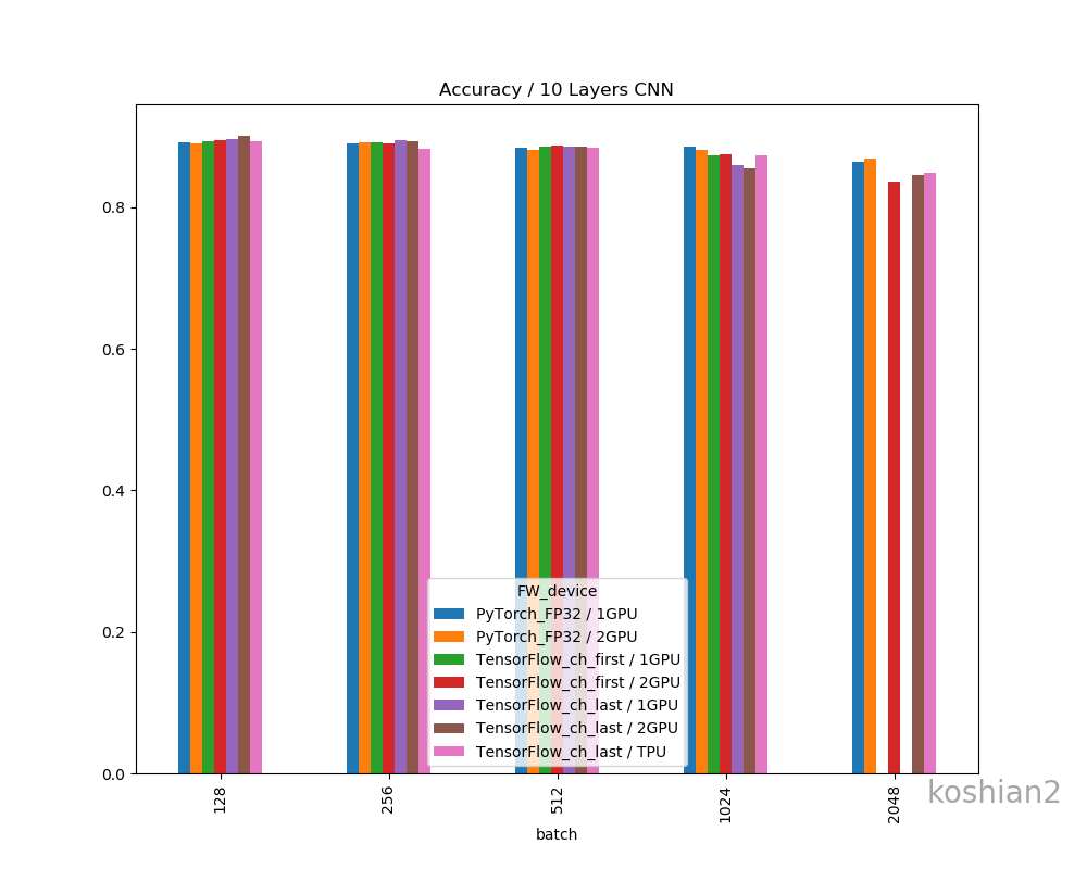
一応、フレームワークやデバイス間で精度の差があるか確認しておきましょう。
精度の明確な差はこのデータだけではなさそうに思えます。明確に議論するならケースごとにもう少し試行回数を増やして精査しないといけません。
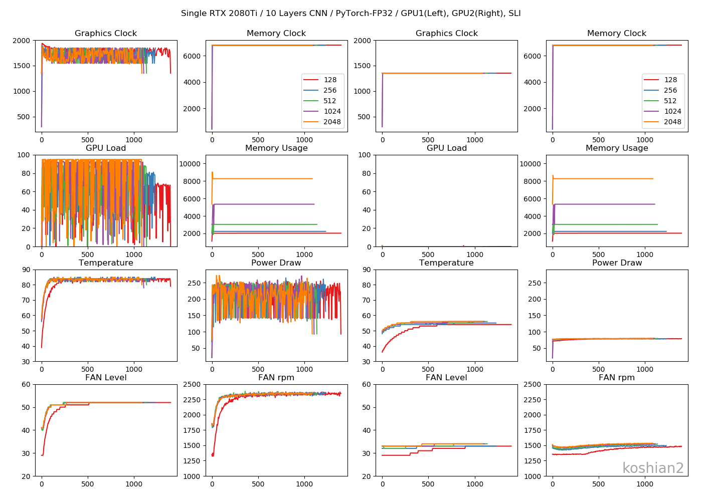
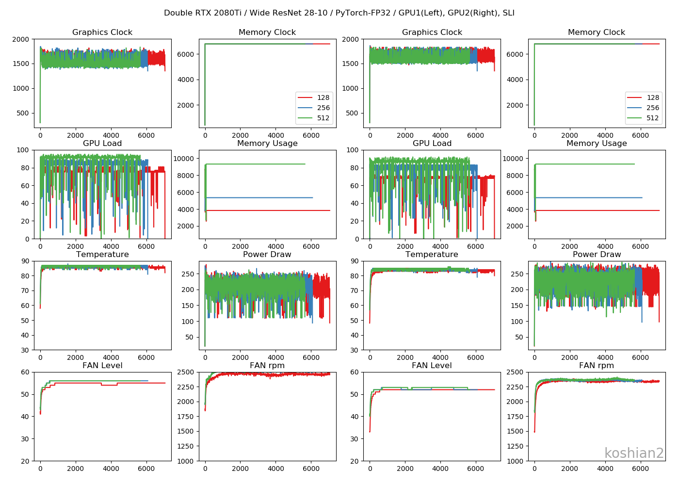
GPUログ
1GPU・10層CNN
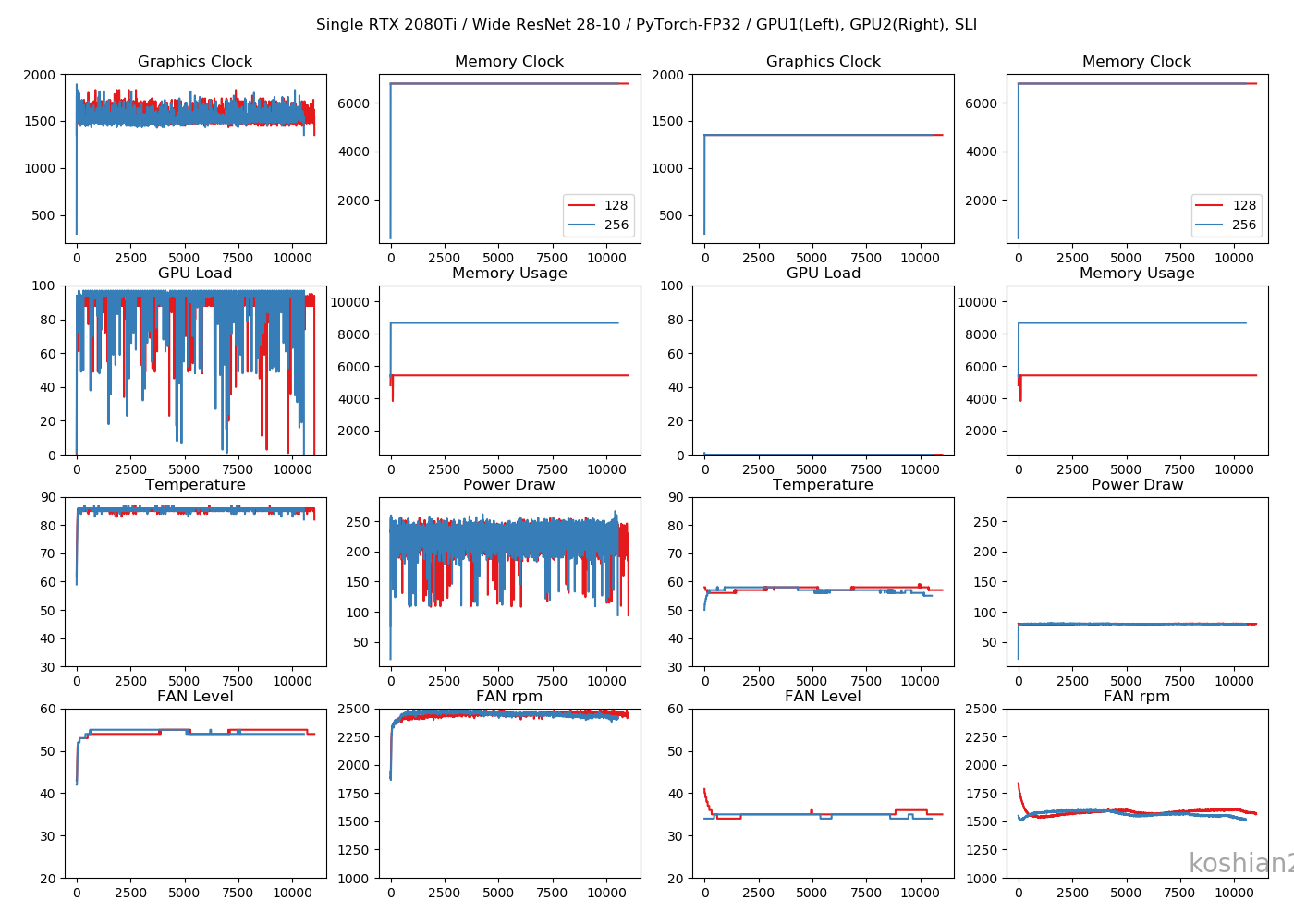
目につくのは「Memory Usage」です。TensorFlowのケースではモデルが大きかろうが小さかろうが、確保できるだけめいいっぱいメモリ確保しているのに対し、PyTorchではモデルに見合ったサイズしかメモリ確保していません。TensorFlowのGPU最適化やっぱりおかしいんじゃ。1GPU・WRN
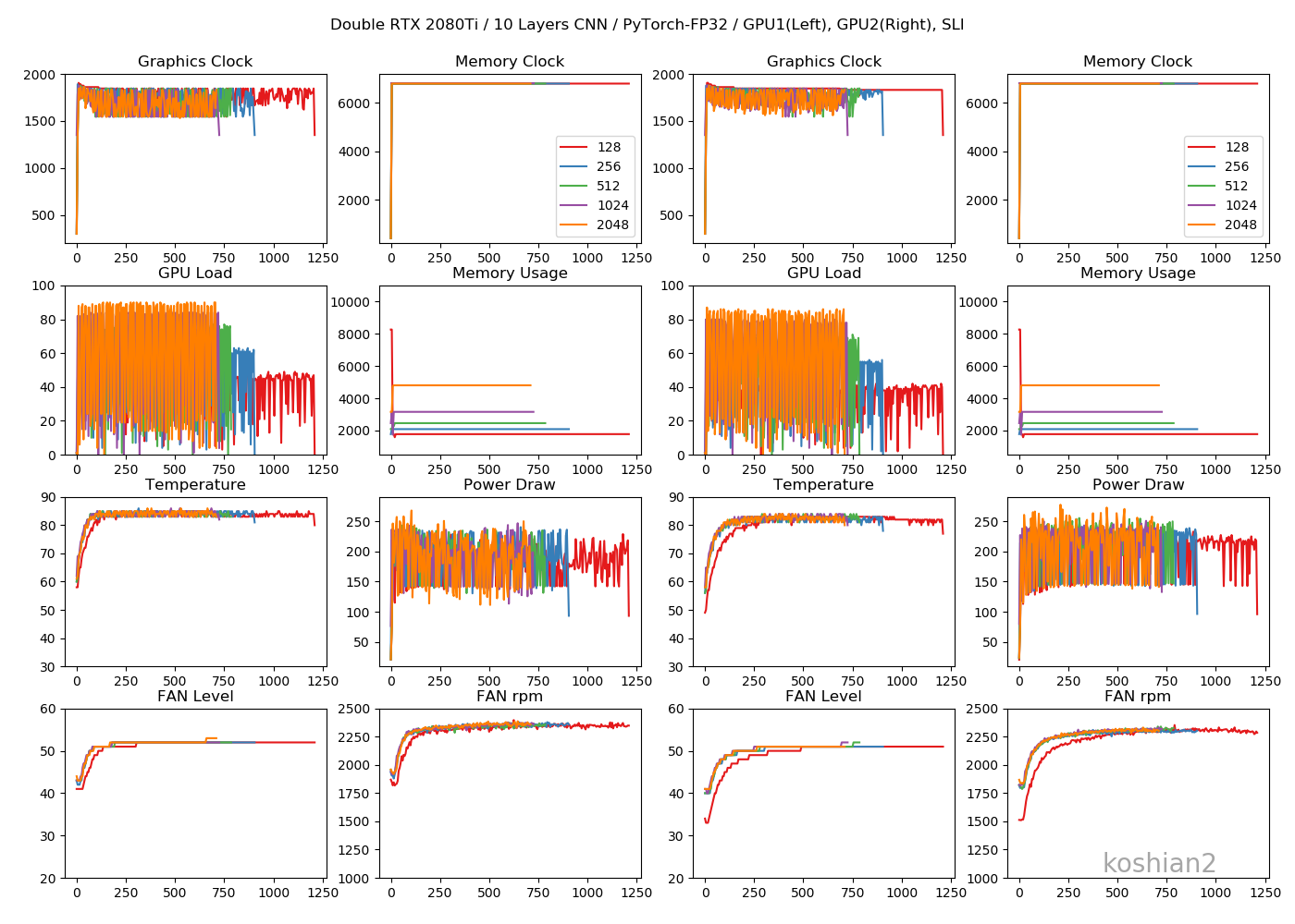
TensorFlowのケースよりGPUロードの振れ幅が大きくなっていますが、これはエポックの終わりで一瞬だけ計算しない時間があるからです。訓練ループを書いているせいもあるかもしれません。2GPU・10層CNN
2GPUの場合は、GPUごとに同じ動きになっていてわかりやすいです。2GPU・WRN
TensorFlowのときにあった、GPUロードの1枚目と2枚目の不均一性は解消されました。これなら自然ですし、速度も出るはずです。まとめ
RTX 2080Ti SLI環境の場合、次のことがわかりました。
- FP32の精度では、1GPUの場合、TensorFlowとPyTorchの速さはあまり変わらない。TensorFlowでchannels_firstにするとPyTorchの速度を上回ることもある。
- ただし、2GPUにするとPyTorchの完勝になる。TensorFlowでは逆に遅くなってしまう。
- 10層CNNのような小さいモデルでは、2GPUのPyTorchにすると、FP32の精度を保ちながらColab TPUより高速化できる。
- ハードウェアが同一なのに、PyTorchのほうが大きなバッチサイズを訓練できることがある。
- PyTorchはモデルの大きさに応じてGPUメモリを専有する。TensorFlow/Kerasは大きいモデルだろうが小さいモデルだろうが、デフォルトでは確保できるだけ確保していて、GPUの最適化がおかしい。
PyTorch with テンソルコアでどれだけ速くなるかは次回に書きたいと思います。
コード
https://gist.github.com/koshian2/f54fe6a4a71f3ba3d68cc2d90c0a3d6d
お知らせ
技術書典6で頒布したモザイク本の通販を下記URLで行っています。会場にこられなかったけど欲しいという方は、ぜひご利用ください。
『DeepCreamPyで学ぶモザイク除去』通販
https://note.mu/koshian2/n/naa60d5c9ebbaディープラーニングや機械学習における画像処理の基本や応用を学びながら、モザイク除去技術DeepCreamPyを使いこなし、自分で実装するまでを目指す解説書です(TPUの実装中心に書いています)。
- 投稿日:2019-05-23T16:50:33+09:00
ElixirでDeep Learning
はじめに
現在、開発中のElixirベースのDeep learningの概要について取りまとめました。プロジェクト名は「Deep Pipe」(DP) といいます。
基本的なアイディア
2つのことを盛り込もうとしています。1つはネットワークの記述につきElixir風の簡易な記述にすること。2つめはElixirの得意分野である並列を活かすことです。
ネットワークの表記
マクロ機能を使って次のようにネットワークを表記します。これはMNISTに対応したものです。
defnetwork init_network4(_x) do
    _x |> f(5,5) |> flatten
    |> w(576,300) |> b(300) |> relu
    |> w(300,100) |> b(100) |> relu
    |> w(100,10) |> b(10) |> sigmoid
  end
f()というのはCNNの畳み込みのフィルタです。f(5,5)ですと5*5のフィルタ行列を生成します。ガウス分布の乱数を生成します。学習率、乗ずる倍数,ストラッド省略可能でありその場合にはそれぞれ0.01, 0.01、1、です。
flattenは行列データを横ベクトルに変換します。CNNから普通のネットワークへの橋渡しです。
例にはありませんが、pad(n), pool(n) があります。paddingとpoolingです。
w()は重み行列です。w(576,300)ですと576*300の行列を生成します。ガウス分布の乱数によっています。オプションで学習率と初期値に対する倍数を設定できます。省略可能です。
b()はバイアスです。要素0の行ベクトルを生成します。学習率は省略可能です。
relu、sigmoidは活性化関数です。
並列
今のところ行列積の計算にSpawnを使った並列処理のものを入れてあります。まだCPUをフルに使いきるところまでいっていません。ミニバッチ学習をプロセスに分割することによりマルチCPUを使い切ることを考えています。Hastegaも取り入れる予定です。
追記
2019/5/25 並列処理によるバックプロパゲーションを追加しました。icore5CPUで使用率が約80%になります。勾配の更新
通常のsgdの他、Momentum、AdaGrad、Adamなどを実装しています。まだ、ハイパーパラメータがうまくつかめていないのか、実装に問題があるのか、まだまだうまく機能していません。
追記2019/5/25
adagradでMNISTにつき93%の正解率まで出せるようになりました。例
MNISTデータを使ってテストをしています。まだまだ実験段階です。
def adam(m,n) do
    IO.puts("preparing data")
    image = MNIST.train_image(2000)
    label = MNIST.train_label_onehot(2000)
    network = Foo.init_network4(0)
    test_image = MNIST.test_image(100)
    test_label = MNIST.test_label(100)
    IO.puts("ready")
    network1 = adam1(image,network,label,m,n)
    correct = accuracy(test_image,network1,test_label,100,0)
    IO.write("accuracy rate = ")
    IO.puts(correct / 100)
  end

  def adam1(_,network,_,_,0) do network end
  def adam1(image,network,train,m,n) do
    {image1,train1} = random_select(image,train,[],[],m)
    network1 = gradient(image1,network,train1)
    network2 = learning(network,network1,:adam)
    y = forward(image1,network2)
    loss = batch_error(y,train1,fn(x,y) -> DP.mean_square(x,y) end)
    DP.print(loss)
    DP.newline()
    adam1(image,network2,train,m,n-1)
  end
全コード
GitHubに置いてあります。
https://github.com/sasagawa888/DeepLearning展望
ようやく基本的な部分が動きつつあるという段階です。これから完成度を上げてきます。今年の後半には完成させたいと思っています。
- 投稿日:2019-05-23T11:59:14+09:00
TensorFlow.jsでDeepLearning(学習用画像データURLの収集)
こんにちわ。Electric Blue Industries Ltd.という、ITで美を追求するファンキーでマニアックなIT企業のマッツと申します。TensorFlow.jsでDeepLearningをする際に学習データ用の画像を収集することがあると思いますが、Google画像検索を使って簡単におこなう小ネタです。
Google画像検索で取得したい画像がリスト表示されたところで、下記のjavascriptをブラウザ(Google Chrome推奨)の開発者ツールのコンソールで実行すると、表示された画像のソースURLがCSVファイルとしてダウンロードできます。
ggl_image_urls.js// 検索結果のHTMLソースから各検索結果のアイテムごとにソースURLを取得し配列化 urls = Array.from(document.querySelectorAll('.rg_di .rg_meta')).map(el=>JSON.parse(el.textContent).ou); // 改行コードを各行末尾に付けたCSVとして吐き出す window.open('data:text/csv;charset=utf-8,' + escape(urls.join('\n')));
追伸: Machine Learning Tokyoと言うMachine Learningの日本最大のグループに参加しています。作業系の少人数会合を中心に顔を出しています。基本的に英語でのコミュニケーションとなっていますが、能力的にも人間的にもトップレベルの素晴らしい方々が参加されておられるので、機会がありましたら参加されることをオススメします。
- 投稿日:2019-05-23T00:32:04+09:00
【画像生成】AutoencoderとVAEと。。。遊んでみた♬
画像生成の基本ということで、MNISTのAutoencoderをやってみました。
一年ちょっと前、参考にあるように中間のLatent_dimの大きさが大きければ得られる画像は入力画像のそれとそん色無いというところまでやりました。
今回は、その先へ。。。今日はVAEとちょっとプラスアルファまでやってみようと思います。
どうやらこの先には大きな宝物が埋まっているかもというところにたどり着いたので、あとの楽しみにしてください。
え??そんなの知っていますという方は、以下は読み飛ばしてください。
【参考】
・CapsNetで遊んでみた♬~Autoencoderと比較すると~やったこと
・MNISTのAutoencoder
・MNISTのVAE
・異常検知について・MNISTのAutoencoder
ここは、いろいろなコードが考えられ、またMNISTには大仰ですが、以下を採用します。
input_img = Input(shape=(28, 28, 1))  # adapt this if using `channels_first` image data format

x = Conv2D(16, (3, 3), activation='relu', padding='same')(input_img)
x = MaxPooling2D((2, 2), padding='same')(x)
x = Conv2D(8, (3, 3), activation='relu', padding='same')(x)
x = MaxPooling2D((2, 2), padding='same')(x)
x = Conv2D(8, (3, 3), activation='relu', padding='same')(x)
encoded = MaxPooling2D((2, 2), padding='same',name='encoded')(x)
encoder=Model(input_img, encoded)
encoder.summary()

x = Conv2D(8, (3, 3), activation='relu', padding='same')(encoded)
x = UpSampling2D((2, 2))(x)
x = Conv2D(8, (3, 3), activation='relu', padding='same')(x)
x = UpSampling2D((2, 2))(x)
x = Conv2D(16, (3, 3), activation='relu')(x)
x = UpSampling2D((2, 2))(x)
decoded = Conv2D(1, (3, 3), activation='sigmoid', padding='same')(x)

autoencoder = Model(input_img, decoded)
autoencoder.compile(optimizer='adadelta', loss='binary_crossentropy')
autoencoder.summary()
ということで結果は以下のとおりになります。
ちなみに変化が見やすいように1000データで10epoch学習して10000個のTestデータで検証しています。
※今回は精度は問いません
コード全体は以下のとおりです。
VAE/AE_mnist_conv2d.py・MNISTのVAE
ここは参考の①②を参考にしています。特に参考①③についてはコードをほぼまんま参考にさせていただきました。また、参考②には詳細な説明があって、VAEとはということが理解できます。
【参考】
①KerasでAutoEncoderその2
②Variational Autoencoder徹底解説
③Example of VAE on MNIST dataset using MLP@KerasDocumentation
こうなると、このあたりやる意味あるのかというですが、ウワン的には上記のAEとこのVAEの差分がどうしても知りたいという欲求にかられました。
ということで、おさらいです。
コードの主要な部分は以下のとおりです。
encoderの最初の部分は通常のencoderと同じです。inputs = Input(shape=input_shape, name='encoder_input') x = Conv2D(16, (3, 3), activation='relu', padding='same')(inputs) x = MaxPooling2D((2, 2), padding='same')(x) x = Conv2D(8, (3, 3), activation='relu', padding='same')(x) x = MaxPooling2D((2, 2), padding='same')(x) x = Conv2D(8, (3, 3), activation='relu', padding='same')(x) x = MaxPooling2D((2, 2), padding='same',name='encoded')(x)以下で最後のTensorの引数を読込み、shapeに格納します。
そして、latent空間でdecoderの出力を制御したいので、以下のようにFlatten()してから、z_meanとz_log_varという分布の平均値と分散の対数に当たる変数を定義します。
この部分がVAEの主な考え方です。
※つまり、ある分布関数(以下で見るように、z=z_mean + K.exp(0.5 * z_log_var) * epsilonという関数)の変数にlatent空間でとる値を制限して制御する
そして例のLambdaクラスを利用して関数定義することにより、Tensorを引き渡す手法を取っています。
こうして、encoderは入力inputs=input_imgに対して、[z_mean, z_log_var]を出力とするモデルとなります。shape = K.int_shape(x) print("shape[1], shape[2], shape[3]",shape[1], shape[2], shape[3]) x = Flatten()(x) z_mean = Dense(latent_dim, name='z_mean')(x) z_log_var = Dense(latent_dim, name='z_log_var')(x) # use reparameterization trick to push the sampling out as input # note that "output_shape" isn't necessary with the TensorFlow backend z = Lambda(sampling, output_shape=(latent_dim,), name='z')([z_mean, z_log_var]) # instantiate encoder model encoder = Model(inputs, [z_mean, z_log_var, z], name='encoder') encoder.summary()一方、decoderは入力は上記のLambdaの出力である[z_mean, z_log_var]の二次元の要素を持ったもので、上記のAutoencoderと同様なモデルです。
# build decoder model
# decoder
latent_inputs = Input(shape=(latent_dim,), name='z_sampling')
x = Dense(shape[1] * shape[2] * shape[3], activation='relu')(latent_inputs)
x = Reshape((shape[1], shape[2], shape[3]))(x)
x = Conv2D(8, (3, 3), activation='relu', padding='same')(x)
x = UpSampling2D((2, 2))(x)
x = Conv2D(8, (3, 3), activation='relu', padding='same')(x)
x = UpSampling2D((2, 2))(x)
x = Conv2D(16, (3, 3), activation='relu')(x)
x = UpSampling2D((2, 2))(x)
outputs = Conv2D(1, (3, 3), activation='sigmoid', padding='same')(x)
# instantiate decoder model
decoder = Model(latent_inputs, outputs, name='decoder')
decoder.summary()
# instantiate VAE model
outputs = decoder(encoder(inputs)[2])
vae = Model(inputs, outputs, name='vae_mlp')
一方、Lambdaが定義していた関数samplingは以下のようなもので、これこそがVAEの肝となるものです。
※参考②のReparameterization Trickあたりを見てください
また、参考③のKerasDocumentationにはこの関数に対して以下のコメントがあります"""Reparameterization trick by sampling for an isotropic unit Gaussian. # Arguments args (tensor): mean and log of variance of Q(z|X) # Returns z (tensor): sampled latent vector """ちなみにGauss分布との関係(すなわちパラメータ変換)については以下が参考になります。
【参考】
Reparameterization Trick for Gaussian Distribution「Assume we have a normal distribution q that is parameterized by θ, specifically $q_θ(x)=N(θ,1)$. We want to solve the below problem
min_θ E_q[x^2]We want to understand how the reparameterization trick helps in calculating the gradient of this objective $E_q[x^2]$.
One way to calculate $∇_θE_q[x^2]$ is as follows
∇_θE_q[x^2]=∇_θ∫q_θ(x)x^2dx=∫x^2∇_θq_θ(x)\frac{q_θ(x)}{q_θ(x)}dx=∫q_θ(x)∇_θ\log q_θ(x)x^2dx
=E_q[x^2∇_θ\log q_θ(x)]
For our example where qθ(x)=N(θ,1), this method gives
∇_θE_q[x2]=E_q[x^2(x−θ)]Reparameterization trick is a way to rewrite the expectation so that the distribution with respect to which we take the expectation is independent of parameter θ. To achieve this, we need to make the stochastic element in q independent of θ. Hence, we write x as
x=θ+ϵ,ϵ∼N(0,1)Then, we can write
E_q[x^2]=E_p[(θ+ϵ)^2]where p is the distribution of ϵ, i.e., N(0,1). Now we can write the derivative of $E_q[x^2]$ as follows
∇_θE_q[x^2]=∇_θE_p[(θ+ϵ)^2]=E_p[2(θ+ϵ)]share cite improve this answer」
def sampling(args):
    z_mean, z_log_var = args
    batch = K.shape(z_mean)[0]
    dim = K.int_shape(z_mean)[1]
    # by default, random_normal has mean=0 and std=1.0
    epsilon = K.random_normal(shape=(batch, dim))
    return z_mean + K.exp(0.5 * z_log_var) * epsilon
最後にVAEのloss関数は以下のとおりです。
# Compute VAE loss
reconstruction_loss = binary_crossentropy(K.flatten(inputs), K.flatten(outputs))
reconstruction_loss *= image_size * image_size
kl_loss = 1 + z_log_var - K.square(z_mean) - K.exp(z_log_var)
kl_loss = K.sum(kl_loss, axis=-1)
kl_loss *= -0.5
vae_loss = K.mean(reconstruction_loss + kl_loss)
そして結果は100epochのとき、以下のとおり得られました。
コード全体は以下のとおりです。
VAE/keras_vae_conv2d.py異常検知について
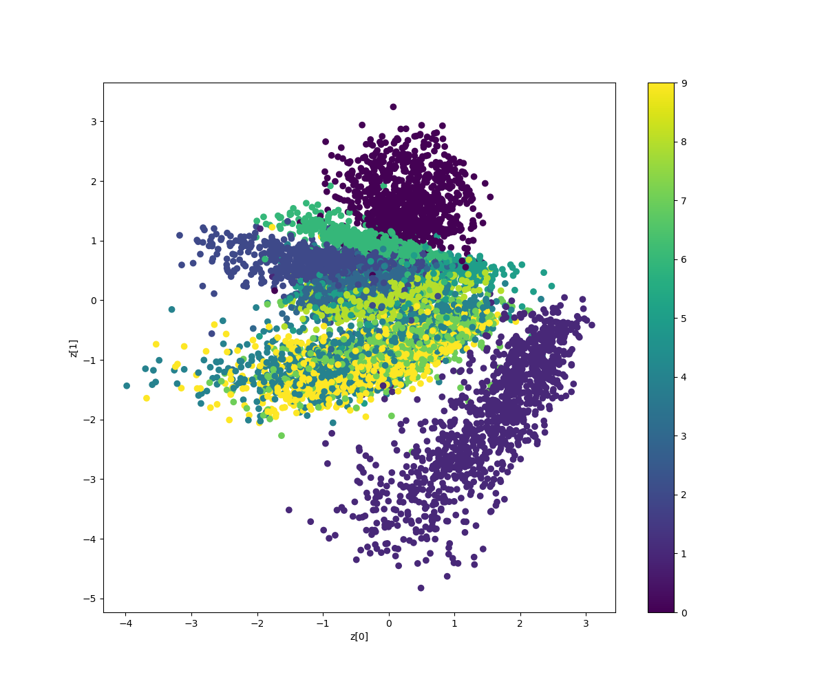
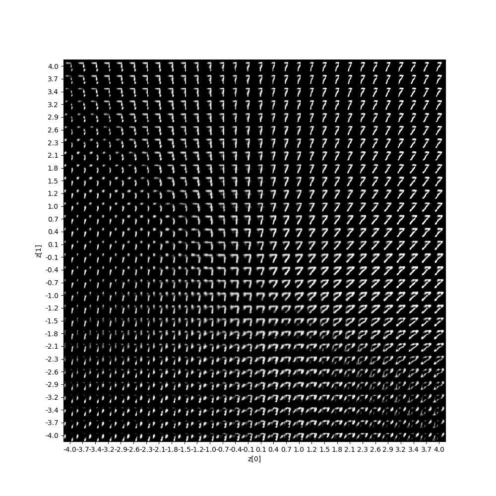
そして参考①で議論されている異常検知、すなわち以下のコードのように学習を7のみに限定して学習すると、そのz空間での様子を見ると以下のようにほぼ全領域で7のような形状になっています。
# 学習に使うデータを限定する
x_train1 = x_train[y_train==7]
x_test1 = x_test[y_test==7]

vae.fit(x_train1,
                epochs=epochs,
                batch_size=batch_size,
                validation_data=(x_test1, None))
そして異常検知の図は以下のとおりになります。
実はここから面白いのですが、この7を学習したモデルでさらに一つずつ文字を学習するとどうなるでしょうか??
DLの記憶って、どうなるか興味がわいたのでやってみましたが、今夜は遅くなったので明日の記事にしたいと思います。まとめ
・Autoencoderをやってみた
・VAEをやってみた
・異常検知についてやってみた・DLの記憶ってあるのかどうか明日書きます

![z_sample_t_No.7_100_50z0=[-0.7,-3]z7=[-0.7,2].gif](https://qiita-image-store.s3.ap-northeast-1.amazonaws.com/0/233744/67942ae9-0958-7a7f-0386-2a874211bea4.gif)

- 投稿日:2019-05-23T00:32:04+09:00
【画像識別】AutoencoderとVAEと。。。遊んでみた♬
画像識別の基本ということで、MNISTのAutoencoderをやってみました。
一年ちょっと前、参考にあるように中間のLatent_dimの大きさが大きければ得られる画像は入力画像のそれとそん色無いというところまでやりました。
今回は、その先へ。。。今日はVAEとちょっとプラスアルファまでやってみようと思います。
どうやらこの先には大きな宝物が埋まっているかもというところにたどり着いたので、あとの楽しみにしてください。
え??そんなの知っていますという方は、以下は読み飛ばしてください。
【参考】
・CapsNetで遊んでみた♬~Autoencoderと比較すると~やったこと
・MNISTのAutoencoder
・MNISTのVAE
・予兆検知について・MNISTのAutoencoder
ここは、いろいろなコードが考えられ、またMNISTには大仰ですが、以下を採用します。
input_img = Input(shape=(28, 28, 1))  # adapt this if using `channels_first` image data format

x = Conv2D(16, (3, 3), activation='relu', padding='same')(input_img)
x = MaxPooling2D((2, 2), padding='same')(x)
x = Conv2D(8, (3, 3), activation='relu', padding='same')(x)
x = MaxPooling2D((2, 2), padding='same')(x)
x = Conv2D(8, (3, 3), activation='relu', padding='same')(x)
encoded = MaxPooling2D((2, 2), padding='same',name='encoded')(x)
encoder=Model(input_img, encoded)
encoder.summary()

x = Conv2D(8, (3, 3), activation='relu', padding='same')(encoded)
x = UpSampling2D((2, 2))(x)
x = Conv2D(8, (3, 3), activation='relu', padding='same')(x)
x = UpSampling2D((2, 2))(x)
x = Conv2D(16, (3, 3), activation='relu')(x)
x = UpSampling2D((2, 2))(x)
decoded = Conv2D(1, (3, 3), activation='sigmoid', padding='same')(x)

autoencoder = Model(input_img, decoded)
autoencoder.compile(optimizer='adadelta', loss='binary_crossentropy')
autoencoder.summary()
ということで結果は以下のとおりになります。
ちなみに変化が見やすいように1000データで10epoch学習して10000個のTestデータで検証しています。
※今回は精度は問いません
コード全体は以下のとおりです。
VAE/AE_mnist_conv2d.py・MNISTのVAE
ここは参考の①②を参考にしています。特に参考①③についてはコードをほぼまんま参考にさせていただきました。また、参考②には詳細な説明があって、VAEとはということが理解できます。
【参考】
①KerasでAutoEncoderその2
②Variational Autoencoder徹底解説
③Example of VAE on MNIST dataset using MLP@KerasDocumentation
こうなると、このあたりやる意味あるのかというですが、ウワン的には上記のAEとこのVAEの差分がどうしても知りたいという欲求にかられました。
ということで、おさらいです。
コードの主要な部分は以下のとおりです。
encoderの最初の部分は通常のencoderと同じです。inputs = Input(shape=input_shape, name='encoder_input') x = Conv2D(16, (3, 3), activation='relu', padding='same')(inputs) x = MaxPooling2D((2, 2), padding='same')(x) x = Conv2D(8, (3, 3), activation='relu', padding='same')(x) x = MaxPooling2D((2, 2), padding='same')(x) x = Conv2D(8, (3, 3), activation='relu', padding='same')(x) x = MaxPooling2D((2, 2), padding='same',name='encoded')(x)以下で最後のTensorの引数を読込み、shapeに格納します。
そして、latent空間でdecoderの出力を制御したいので、以下のようにFlatten()してから、z_meanとz_log_varという分布の平均値と分散の対数に当たる変数を定義します。
この部分がVAEの主な考え方です。
※つまり、ある分布関数(以下で見るように、z=z_mean + K.exp(0.5 * z_log_var) * epsilonという関数)の変数にlatent空間でとる値を制限して制御する
そして例のLambdaクラスを利用して関数定義することにより、Tensorを引き渡す手法を取っています。
こうして、encoderは入力inputs=input_imgに対して、[z_mean, z_log_var]を出力とするモデルとなります。shape = K.int_shape(x) print("shape[1], shape[2], shape[3]",shape[1], shape[2], shape[3]) x = Flatten()(x) z_mean = Dense(latent_dim, name='z_mean')(x) z_log_var = Dense(latent_dim, name='z_log_var')(x) # use reparameterization trick to push the sampling out as input # note that "output_shape" isn't necessary with the TensorFlow backend z = Lambda(sampling, output_shape=(latent_dim,), name='z')([z_mean, z_log_var]) # instantiate encoder model encoder = Model(inputs, [z_mean, z_log_var, z], name='encoder') encoder.summary()一方、decoderは入力は上記のLambdaの出力である[z_mean, z_log_var]の二次元の要素を持ったもので、上記のAutoencoderと同様なモデルです。
# build decoder model
# decoder
latent_inputs = Input(shape=(latent_dim,), name='z_sampling')
x = Dense(shape[1] * shape[2] * shape[3], activation='relu')(latent_inputs)
x = Reshape((shape[1], shape[2], shape[3]))(x)
x = Conv2D(8, (3, 3), activation='relu', padding='same')(x)
x = UpSampling2D((2, 2))(x)
x = Conv2D(8, (3, 3), activation='relu', padding='same')(x)
x = UpSampling2D((2, 2))(x)
x = Conv2D(16, (3, 3), activation='relu')(x)
x = UpSampling2D((2, 2))(x)
outputs = Conv2D(1, (3, 3), activation='sigmoid', padding='same')(x)
# instantiate decoder model
decoder = Model(latent_inputs, outputs, name='decoder')
decoder.summary()
# instantiate VAE model
outputs = decoder(encoder(inputs)[2])
vae = Model(inputs, outputs, name='vae_mlp')
一方、Lambdaが定義していた関数samplingは以下のようなもので、これこそがVAEの肝となるものです。
※参考②のReparameterization Trickあたりを見てください
また、参考③のKerasDocumentationにはこの関数に対して以下のコメントがあります"""Reparameterization trick by sampling for an isotropic unit Gaussian. # Arguments args (tensor): mean and log of variance of Q(z|X) # Returns z (tensor): sampled latent vector """ちなみにGauss分布との関係(すなわちパラメータ変換)については以下が参考になります。
【参考】
Reparameterization Trick for Gaussian Distribution「Assume we have a normal distribution q that is parameterized by θ, specifically $q_θ(x)=N(θ,1)$. We want to solve the below problem
min_θ E_q[x^2]We want to understand how the reparameterization trick helps in calculating the gradient of this objective $E_q[x^2]$.
One way to calculate $∇_θE_q[x^2]$ is as follows
∇_θE_q[x^2]=∇_θ∫q_θ(x)x^2dx=∫x^2∇_θq_θ(x)\frac{q_θ(x)}{q_θ(x)}dx=∫q_θ(x)∇_θ\log q_θ(x)x^2dx
=E_q[x^2∇_θ\log q_θ(x)]
For our example where qθ(x)=N(θ,1), this method gives
∇_θE_q[x2]=E_q[x^2(x−θ)]Reparameterization trick is a way to rewrite the expectation so that the distribution with respect to which we take the expectation is independent of parameter θ. To achieve this, we need to make the stochastic element in q independent of θ. Hence, we write x as
x=θ+ϵ,ϵ∼N(0,1)Then, we can write
E_q[x^2]=E_p[(θ+ϵ)^2]where p is the distribution of ϵ, i.e., N(0,1). Now we can write the derivative of $E_q[x^2]$ as follows
∇_θE_q[x^2]=∇_θE_p[(θ+ϵ)^2]=E_p[2(θ+ϵ)]share cite improve this answer」
def sampling(args):
    z_mean, z_log_var = args
    batch = K.shape(z_mean)[0]
    dim = K.int_shape(z_mean)[1]
    # by default, random_normal has mean=0 and std=1.0
    epsilon = K.random_normal(shape=(batch, dim))
    return z_mean + K.exp(0.5 * z_log_var) * epsilon
最後にVAEのloss関数は以下のとおりです。
# Compute VAE loss
reconstruction_loss = binary_crossentropy(K.flatten(inputs), K.flatten(outputs))
reconstruction_loss *= image_size * image_size
kl_loss = 1 + z_log_var - K.square(z_mean) - K.exp(z_log_var)
kl_loss = K.sum(kl_loss, axis=-1)
kl_loss *= -0.5
vae_loss = K.mean(reconstruction_loss + kl_loss)
そして結果は100epochのとき、以下のとおり得られました。
コード全体は以下のとおりです。
VAE/keras_vae_conv2d.py異常検知について
そして参考①で議論されている異常検知、すなわち以下のコードのように学習を7のみに限定して学習すると、そのz空間での様子を見ると以下のようにほぼ全領域で7のような形状になっています。
# 学習に使うデータを限定する
x_train1 = x_train[y_train==7]
x_test1 = x_test[y_test==7]

vae.fit(x_train1,
                epochs=epochs,
                batch_size=batch_size,
                validation_data=(x_test1, None))
そして異常検知の図は以下のとおりになります。
実はここから面白いのですが、この7を学習したモデルでさらに一つずつ文字を学習するとどうなるでしょうか??
DLの記憶って、どうなるか興味がわいたのでやってみましたが、今夜は遅くなったので明日の記事にしたいと思います。まとめ
・Autoencoderをやってみた
・VAEをやってみた
・異常検知についてやってみた・DLの記憶ってあるのかどうか明日書きます