- 投稿日:2020-05-27T13:22:04+09:00
TensorFlowの画像識別モデルをTensorFlow-TensorRTで推論高速化
NVIDIAの大串です。今回はDeep Learning(TensorFlow)の推論をGPUで実行する際に高速化ができるTensorFlow-TensorRTに関して記事を書かせて頂きました。
モチベーション
Deep Learningモデルの推論は計算量が多いため、通常の処理に比べ時間がかかるケースが多いです。ユースケースによっては厳しい時間制約の中でDeep Learningモデルの推論結果が求められます。
このようなケースに対応するため、NVIDIAはGPUでDeep Learningモデルの推論処理を高速化できるTensorRTライブラリを開発しています。
TensorRTはTensorFlowに統合されており、TensorFlowから簡単に呼び出すことができます。これはTensorFlow-TensorRT(以下:略称TF-TRT)と呼ばれて、TensorFlowの便利な機能をそのまま使えます。詳細は後述します。TensorRTとは
GPU上でのDeep Learningの推論処理を高速化するライブラリです。
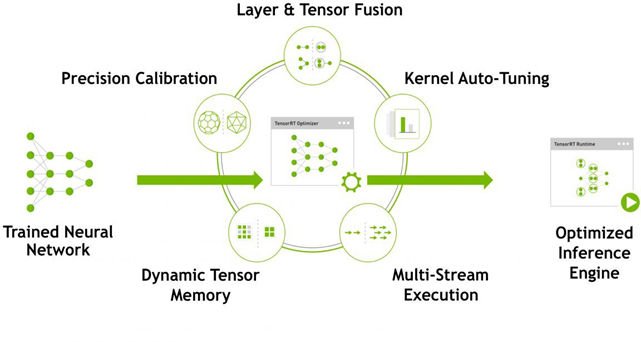
内部では下記の処理をしています。
- レイヤー&テンソル合成
- 数値精度調整
- 自動カーネルチューニング
- 動的テンソルメモリの確保
- 複数ストリーム実行
レイヤー&テンソル合成
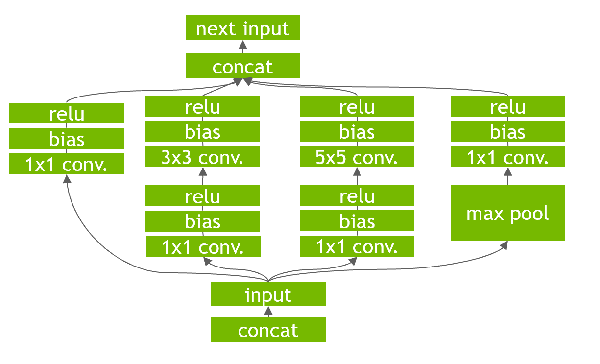
レイヤー&テンソル合成は、与えられたネットワークに対して、垂直合成、水平合成、レイヤー除去を行う処理です。例えば、
上記のようなネットワークが与えられたとき、それぞれ以下の処理が行われます。
- 垂直合成:上記の図は、通常は畳み込み層の後にバイアス、活性化関数が存在しています。それぞれでGPUに対してカーネル命令を発行すると効率的でないため、1つにまとめることでカーネル命令の発行を効率化しています。
- 水平合成:上記の図だと1x1畳み込みが複数存在しています。こちらも垂直統合と同様にそれぞれでGPUカーネル命令を発行するとオーバーヘッドがかかるため、同一の処理をまとめる水平合成を行います。
- レイヤー除去:TensorRTは、出力バッファーを事前に割り当て、ストライド方式でそれらに書き込むことにより、concat層を排除することもできます。これによって余分なオーバーヘッドを避けられます。
なお注意点としてプルーニングとは異なり、精度への寄与が少ないノードを削除する処理ではありません。
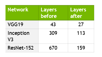
下記の図はレイヤー合成の結果になります。
実際にどの程度レイヤーが削減されるかを下記の図で示します。最大で76%程度削減しています。
数値精度調整
FP32、FP16、INT8と数値精度の調整が可能です。
FP16、INT8を使用する場合はTensorコアを搭載したGPUであればより高速に動作します。
TensorコアについてはAutomatic Mixed Precision (AMP) でニューラルネットワークのトレーニングを高速化をご参照ください。
INT8に関して
INT8はFP16に比べ、大幅にデータの表現する範囲が変わるためキャリブレーションデータによる調整が必要になります。
INT8への変換による精度低下を防ぐためには、元の数値範囲のどこからどこまでをINT8の範囲にマッピングするか、という閾値を設ける必要があります。この閾値は、キャリブレーションデータによって調整されます。
キャリブレーションは下記の方法で行われます。
- 活性化関数の出力でヒストグラムを作成します
- 複数の閾値を用いて量子化します
- それぞれ量子化前と比較してKL Divergenceを計算します
- 最小になる閾値を最終的な結果にします
さらに詳細な情報を把握したい方は8-bit Inference with TensorRTをご参照ください。
自動カーネルチューニング
対象となるGPUごとに以下のようなパラメータの最適値が異なるので最適なカーネルを自動的に選択します。
- バッチサイズ
- 入力サイズ
- バッファーサイズ
- etc
動的Tensorメモリの確保
TensorRTは、実行中のみ使用する各テンソルのメモリを指定することにより、メモリフットプリントを削減し、メモリの再利用を改善し、高速かつ効率的な実行のためのメモリ割り当てオーバーヘッドを回避します。
参考:TensorRT 3: Faster TensorFlow Inference and Volta Support
複数ストリーム実行
作成されたTensorRTエンジンは複数の実行コンテキストを持つことができ、1セットの重みを複数の重複する推論タスクに使用できます。
たとえば、ストリームごとに1つのエンジンと1つのコンテキストを使用して、並列CUDAストリームで画像を処理できます。 各コンテキストは、TensorRTエンジンと同じGPUで作成されます。参考:NVIDIA TensorRT Documentation
TensorFlowにプラグインされたTensorRT
通常のTensorRTと異なる点
TensorFlowのAPIに統合されており、変換処理が簡単に実行可能です。わずかな労力で推論のパフォーマンスが最大8倍向上します。
- TensorFlowにインテグレートされており、下記のモジュールに設定されています。(2020年6月3日時点)
TensorFlowのエコシステムが利用可能なため、TensorFlow Python APIやJupyterノートブックを引き続き使用可能です。
- TensorBoardが利用可能なため、TensorFlow-TensorRTで変換後のモデルを確認できます。
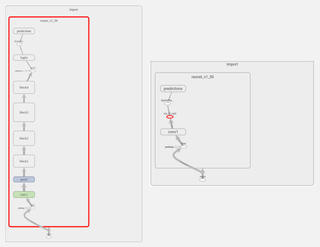
- 下記の図はTensorBoard上でTF-TRTで最適化する前のグラフ(左)と最適化後のグラフ(右)を確認した結果になります。参考:TensorRT Integration Speeds Up TensorFlow Inference
- 左:最適化前のモデル、右:最適化後のモデル
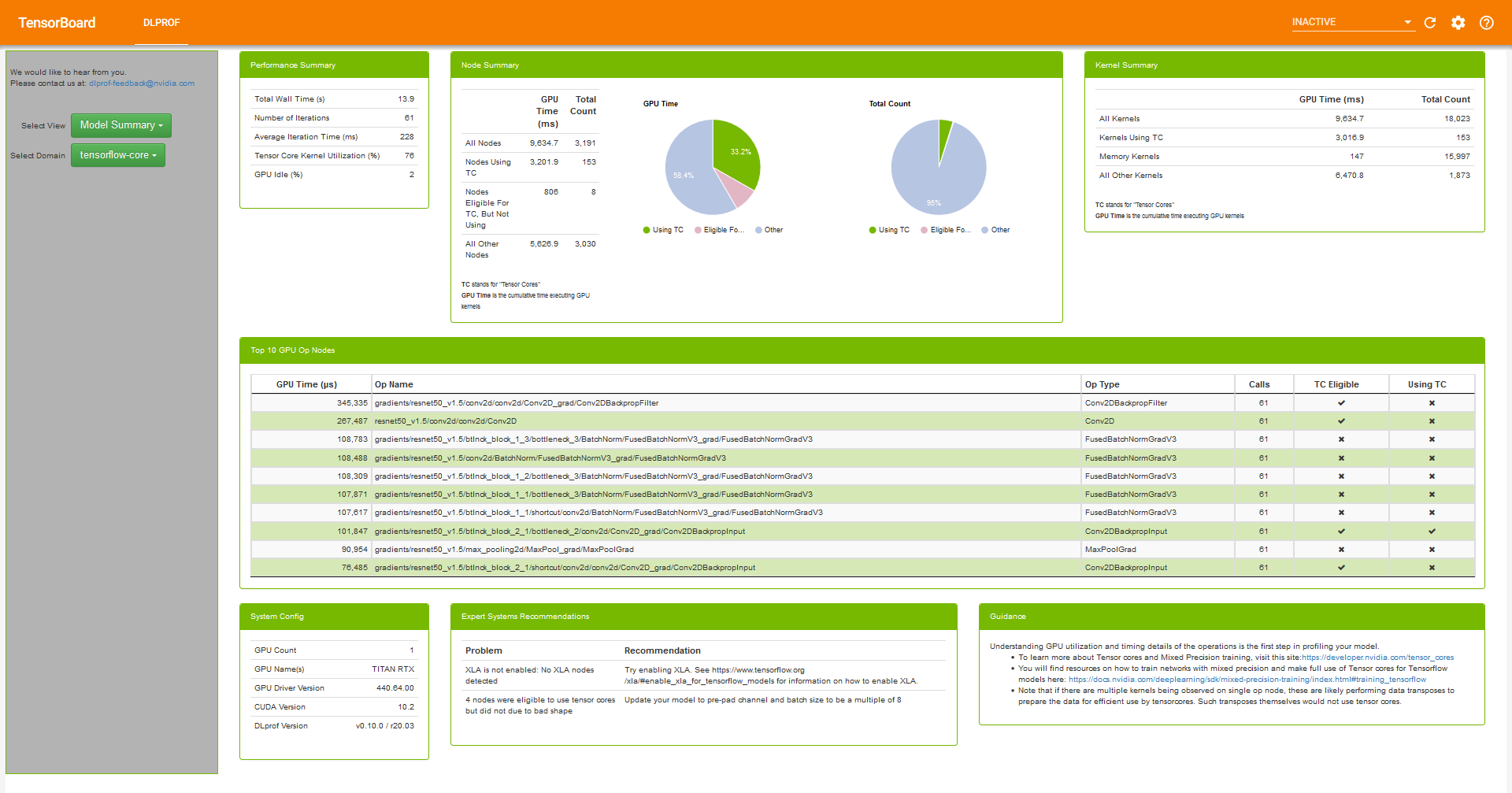
- TensorBoardにプラグインされた機能であるDLProfを使用して詳細な情報を知ることができます。これによってTensorコアの使用率や各オぺレーションごとのGPU使用時間などを知ることができます。
- 参考:Deep Learning Profiler (DLProf) User Guide
TensorRTがサポートしていないレイヤーはTensorFlowへフォールバックするため、TensorRTでカスタムレイヤーの記述が必要なモデルも対応可能です。
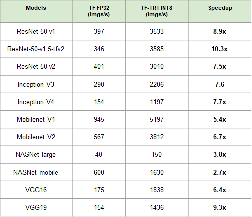
パフォーマンス
こちらのパフォーマンス情報はTensorRT inference with TensorFlow 2.0から引用しています。
画像識別モデルのスループットは下記になります。最大10倍程度の性能向上しています。
検証環境は下記になります。
- GPU: NVIDIA T4
- 数値精度:INT8
- バッチサイズ 32
- I/Oの時間は考慮しない
- TensorFLow: 2.1.0
- TensorRT: 7.0.0
- 使用しているdocker: Tensorflow 20.02-tf2-py3
- 実行スクリプト(2020年3月時点のコード):image_classification.py
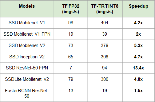
物体検出モデルのスループットは下記になります。最大13倍程度の性能向上しています。
検証環境は下記になります。
- GPU: NVIDIA T4
- 数値精度:INT8
- バッチサイズ 32
- I/Oの時間は考慮しない
- TensorFLow: 2.1.0
- TensorRT: 7.0.0
- 使用しているdocker: Tensorflow 20.02-tf2-py3
- 実行スクリプト(2020年3月時点のコード):image_classification.py
さらに詳細なパフォーマンスに関してはNVIDIA Data Center Deep Learning Product Performanceをご覧ください。
TF-TRTの使用方法
Google ColaboratoryのGPU環境で動作検証しました。
使用するGPUの確認します。今回はNVIDIA P100のGPUを使用しています。
Mon May 25 01:46:10 2020
+-----------------------------------------------------------------------------+
| NVIDIA-SMI 440.82       Driver Version: 418.67       CUDA Version: 10.1     |
|-------------------------------+----------------------+----------------------+
| GPU  Name        Persistence-M| Bus-Id        Disp.A | Volatile Uncorr. ECC |
| Fan  Temp  Perf  Pwr:Usage/Cap|         Memory-Usage | GPU-Util  Compute M. |
|===============================+======================+======================|
|   0  Tesla P100-PCIE...  Off  | 00000000:00:04.0 Off |                    0 |
| N/A   46C    P0    30W / 250W |      0MiB / 16280MiB |      0%      Default |
+-------------------------------+----------------------+----------------------+

+-----------------------------------------------------------------------------+
| Processes:                                                       GPU Memory |
|  GPU       PID   Type   Process name                             Usage      |
|=============================================================================|
|  No running processes found                                                 |
+-----------------------------------------------------------------------------+
コードは下記のgithubで公開されているコードを元に説明します。(2020年1月10日公開のコード)
Google Colaboratoryでの環境構築
TensorFlowのバージョンを2.0.0に変更して、
pillow、matplotlibを導入します。!pip install pillow matplotlib !pip install tensorflow-gpu==2.0.0TF-TRTから使用するTensorRTのバージョンはTensorFlowのバージョンごとに異なるため、TensorFlow 2.0.0で使用可能なTensorRTを導入しています。
%%bash
wget https://developer.download.nvidia.com/compute/machine-learning/repos/ubuntu1804/x86_64/nvidia-machine-learning-repo-ubuntu1804_1.0.0-1_amd64.deb

dpkg -i nvidia-machine-learning-repo-*.deb
apt-get update

sudo apt-get install libnvinfer5
対象のGPUで、Tensorコアが利用可能かどうかを確認します。これが見つからない場合はFP16、INT8のような数値精度で性能が十分に向上しないケースがあります。
from tensorflow.python.client import device_lib

def check_tensor_core_gpu_present():
    local_device_protos = device_lib.list_local_devices()
    for line in local_device_protos:
        if "compute capability" in str(line):
            compute_capability = float(line.physical_device_desc.split("compute capability: ")[-1])
            if compute_capability>=7.0:
                return True

print("Tensor Core GPU Present:", check_tensor_core_gpu_present())
tensor_core_gpu = check_tensor_core_gpu_present()
P100 GPUにはTensorコアが存在していません。
Tensor Core GPU Present: None必要なライブラリをインポートします。
from __future__ import absolute_import, division, print_function, unicode_literals
import os
import time

import numpy as np
import matplotlib.pyplot as plt

import tensorflow as tf
from tensorflow import keras
from tensorflow.python.compiler.tensorrt import trt_convert as trt
from tensorflow.python.saved_model import tag_constants
from tensorflow.keras.applications.resnet50 import ResNet50
from tensorflow.keras.preprocessing import image
from tensorflow.keras.applications.resnet50 import preprocess_input, decode_predictions
データの準備
推論処理用のデータを取得します。
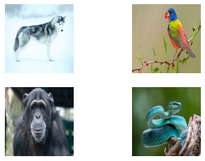
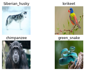
!mkdir ./data
!wget  -O ./data/img0.JPG "https://d17fnq9dkz9hgj.cloudfront.net/breed-uploads/2018/08/siberian-husky-detail.jpg?bust=1535566590&width=630"
!wget  -O ./data/img1.JPG "https://www.hakaimagazine.com/wp-content/uploads/header-gulf-birds.jpg"
!wget  -O ./data/img2.JPG "https://www.artis.nl/media/filer_public_thumbnails/filer_public/00/f1/00f1b6db-fbed-4fef-9ab0-84e944ff11f8/chimpansee_amber_r_1920x1080.jpg__1920x1080_q85_subject_location-923%2C365_subsampling-2.jpg"
!wget  -O ./data/img3.JPG "https://www.familyhandyman.com/wp-content/uploads/2018/09/How-to-Avoid-Snakes-Slithering-Up-Your-Toilet-shutterstock_780480850.jpg"
データの確認をします。
from tensorflow.keras.preprocessing import image

fig, axes = plt.subplots(nrows=2, ncols=2)

for i in range(4):
  img_path = './data/img%d.JPG'%i
  img = image.load_img(img_path, target_size=(224, 224))
  plt.subplot(2,2,i+1)
  plt.imshow(img);
  plt.axis('off');
TensorFlow モデル
ここからはTensorFlowに統合されたKerasモジュールをTF-Kerasと表記して説明させていただきます。
TF-KerasのResNet50の学習済みモデルを取得します。
model = ResNet50(weights='imagenet')まずTF-Kerasのモデルに対して直接、予測処理を行わせてみましょう。
for i in range(4):
  img_path = './data/img%d.JPG'%i
  img = image.load_img(img_path, target_size=(224, 224))
  x = image.img_to_array(img)
  x = np.expand_dims(x, axis=0)
  x = preprocess_input(x)

  preds = model.predict(x)
  # decode the results into a list of tuples (class, description, probability)
  # (one such list for each sample in the batch)
  print('{} - Predicted: {}'.format(img_path, decode_predictions(preds, top=3)[0]))

  plt.subplot(2,2,i+1)
  plt.imshow(img);
  plt.axis('off');
  plt.title(decode_predictions(preds, top=3)[0][0][1])
すべての画像が下記のように正しく認識されていることが分かります。
./data/img0.JPG - Predicted: [('n02110185', 'Siberian_husky', 0.5566208), ('n02109961', 'Eskimo_dog', 0.4173726), ('n02110063', 'malamute', 0.020951567)]
./data/img1.JPG - Predicted: [('n01820546', 'lorikeet', 0.30138937), ('n01537544', 'indigo_bunting', 0.16979575), ('n01828970', 'bee_eater', 0.16134149)]
./data/img2.JPG - Predicted: [('n02481823', 'chimpanzee', 0.51498646), ('n02480495', 'orangutan', 0.15896705), ('n02480855', 'gorilla', 0.15318157)]
./data/img3.JPG - Predicted: [('n01729977', 'green_snake', 0.42379653), ('n03627232', 'knot', 0.09050951), ('n01749939', 'green_mamba', 0.06557772)]
TF-TRTによる最適化処理を行うため、取得した学習済みモデルをSavedModel形式で保存します。
# Save the entire model as a SavedModel.
model.save('resnet50_saved_model')
保存されたモデルの情報を確認します。
!saved_model_cli show --all --dir resnet50_saved_model
serving_defaultの部分に予測モデルの入力と出力の情報があります。この情報はTF-TRTでモデルの読み込み、予測する際に必要な情報になります。MetaGraphDef with tag-set: 'serve' contains the following SignatureDefs: signature_def['__saved_model_init_op']: The given SavedModel SignatureDef contains the following input(s): The given SavedModel SignatureDef contains the following output(s): outputs['__saved_model_init_op'] tensor_info: dtype: DT_INVALID shape: unknown_rank name: NoOp Method name is: signature_def['serving_default']: The given SavedModel SignatureDef contains the following input(s): inputs['input_1'] tensor_info: dtype: DT_FLOAT shape: (-1, 224, 224, 3) name: serving_default_input_1:0 The given SavedModel SignatureDef contains the following output(s): outputs['probs'] tensor_info: dtype: DT_FLOAT shape: (-1, 1000) name: StatefulPartitionedCall:0 Method name is: tensorflow/serving/predictTensorFlowモデルのパフォーマンス
先程保存したモデルを読み込みます。
model = tf.keras.models.load_model('resnet50_saved_model')推論結果が正しいか確認します。
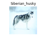
Siberian_huskyを正しく認識できていることが分かります。img_path = './data/img0.JPG' # Siberian_husky img = image.load_img(img_path, target_size=(224, 224)) x = image.img_to_array(img) x = np.expand_dims(x, axis=0) x = preprocess_input(x) preds = model.predict(x) # decode the results into a list of tuples (class, description, probability) # (one such list for each sample in the batch) print('{} - Predicted: {}'.format(img_path, decode_predictions(preds, top=3)[0])) plt.subplot(2,2,1) plt.imshow(img); plt.axis('off'); plt.title(decode_predictions(preds, top=3)[0][0][1])./data/img0.JPG - Predicted: [('n02110185', 'Siberian_husky', 0.55662084), ('n02109961', 'Eskimo_dog', 0.41737264), ('n02110063', 'malamute', 0.02095159)] Text(0.5, 1.0, 'Siberian_husky')
今回のベンチマークでは、一例としてバッチサイズ8を対象とするため、画像を前処理し、バッチを構築します。
batch_size = 8
batched_input = np.zeros((batch_size, 224, 224, 3), dtype=np.float32)

for i in range(batch_size):
  img_path = './data/img%d.JPG' % (i % 4)
  img = image.load_img(img_path, target_size=(224, 224))
  x = image.img_to_array(img)
  x = np.expand_dims(x, axis=0)
  x = preprocess_input(x)
  batched_input[i, :] = x
batched_input = tf.constant(batched_input)
print('batched_input shape: ', batched_input.shape)
ここではベンチマークとして、Throughputを指標とした計測を行います。
安定した状態の性能を計測するため、ベンチマークを取る場合は複数回実行してからベンチマークを取っています。
# Benchmarking throughput
N_warmup_run = 50
N_run = 1000
elapsed_time = []

for i in range(N_warmup_run):
  preds = model.predict(batched_input)

for i in range(N_run):
  start_time = time.time()
  preds = model.predict(batched_input)
  end_time = time.time()
  elapsed_time = np.append(elapsed_time, end_time - start_time)
  if i % 50 == 0:
    print('Step {}: {:4.1f}ms'.format(i, (elapsed_time[-50:].mean()) * 1000))

print('Throughput: {:.0f} images/s'.format(N_run * batch_size / elapsed_time.sum()))
下記の結果
Throughputは1秒間に処理できる画像数になるので、値が大きいほどよい結果になります。Throughput: 226 images/sTF-TRT FP32のモデル
ここから、TF-TRTによるモデルの変換を行います。はじめに、FP32での変換です。
max_workspace_size_bytesはTensorRTが使用可能な最大のGPUメモリサイズを設定しています。TensorRTに変換されるノードが多いほど、この値を大きくしておくと速度アップが行えます。ただし大きくしすぎるとモデルのTensorRT変換が失敗してしまいます。モデル、使用するGPUによって適切なサイズが異なります。print('Converting to TF-TRT FP32...') conversion_params = trt.DEFAULT_TRT_CONVERSION_PARAMS._replace(precision_mode=trt.TrtPrecisionMode.FP32, max_workspace_size_bytes=8000000000) converter = trt.TrtGraphConverterV2(input_saved_model_dir='resnet50_saved_model', conversion_params=conversion_params) converter.convert() converter.save(output_saved_model_dir='resnet50_saved_model_TFTRT_FP32') print('Done Converting to TF-TRT FP32')下記のコマンドでTF-TRTで変換後のモデルを利用するために必要となる、グラフと出力ラベルの情報を確認します。
!saved_model_cli show --all --dir resnet50_saved_model_TFTRT_FP32出力結果を確認します。
serving_defaultに予測するモデルの情報があります。probに予測結果の情報があります。MetaGraphDef with tag-set: 'serve' contains the following SignatureDefs: signature_def['__saved_model_init_op']: The given SavedModel SignatureDef contains the following input(s): The given SavedModel SignatureDef contains the following output(s): outputs['__saved_model_init_op'] tensor_info: dtype: DT_INVALID shape: unknown_rank name: NoOp Method name is: signature_def['serving_default']: The given SavedModel SignatureDef contains the following input(s): inputs['input_1'] tensor_info: dtype: DT_FLOAT shape: (-1, 224, 224, 3) name: serving_default_input_1:0 The given SavedModel SignatureDef contains the following output(s): outputs['probs'] tensor_info: dtype: DT_FLOAT shape: unknown_rank name: PartitionedCall:0 Method name is: tensorflow/serving/predictTF-TRT の数値精度FP32で予測を行います。
上記コマンドの通り、tag-set: 'serve'のモデルが今回の処理対象となるため、TF-TRTで最適化されたモデルを読み込む際にtagsをtag_constants.SERVINGに設定してグラフを読み込みます。上記のコマンドで
serving_defaultに予測モデルの情報があることを確認したのでinfer = saved_model_loaded.signatures['serving_default']で予測モデルを取得します。上記のコマンドで
probsに出力結果があることがわかるのでpreds = labeling['probs'].numpy()で取得します。def predict_tftrt(input_saved_model): """Runs prediction on a single image and shows the result. input_saved_model (string): Name of the input model stored in the current dir """ img_path = './data/img0.JPG' # Siberian_husky img = image.load_img(img_path, target_size=(224, 224)) x = image.img_to_array(img) x = np.expand_dims(x, axis=0) x = preprocess_input(x) x = tf.constant(x) saved_model_loaded = tf.saved_model.load(input_saved_model, tags=[tag_constants.SERVING]) signature_keys = list(saved_model_loaded.signatures.keys()) print(signature_keys) infer = saved_model_loaded.signatures['serving_default'] print(infer.structured_outputs) labeling = infer(x) preds = labeling['probs'].numpy() print('{} - Predicted: {}'.format(img_path, decode_predictions(preds, top=3)[0])) plt.subplot(2,2,1) plt.imshow(img); plt.axis('off'); plt.title(decode_predictions(preds, top=3)[0][0][1])通常のTensorFlowモデルと同様にベンチマークを行います。
def benchmark_tftrt(input_saved_model): saved_model_loaded = tf.saved_model.load(input_saved_model, tags=[tag_constants.SERVING]) infer = saved_model_loaded.signatures['serving_default'] N_warmup_run = 50 N_run = 1000 elapsed_time = [] for i in range(N_warmup_run): labeling = infer(batched_input) for i in range(N_run): start_time = time.time() labeling = infer(batched_input) #prob = labeling['probs'].numpy() end_time = time.time() elapsed_time = np.append(elapsed_time, end_time - start_time) if i % 50 == 0: print('Step {}: {:4.1f}ms'.format(i, (elapsed_time[-50:].mean()) * 1000)) print('Throughput: {:.0f} images/s'.format(N_run * batch_size / elapsed_time.sum()))
Throughputは3.2倍程度上がっています。Throughput: 727 images/sTF-TRT FP16のモデル
githubには記述されていませんが、一度TFTRTの変換を実行したNotebookでは、2回目以降の変換が適切に実行されないことがあるため、Notebookを再起動します。
import os os.kill(os.getpid(), 9)Notebookを再起動したのでライブラリをインポートします。
from __future__ import absolute_import, division, print_function, unicode_literals import os import time import numpy as np import matplotlib.pyplot as plt import tensorflow as tf from tensorflow import keras from tensorflow.python.compiler.tensorrt import trt_convert as trt from tensorflow.python.saved_model import tag_constants from tensorflow.keras.applications.resnet50 import ResNet50 from tensorflow.keras.preprocessing import image from tensorflow.keras.applications.resnet50 import preprocess_input, decode_predictionsTF-TRTのFP32と同様のコードでデータの前処理を行います。
batch_size = 8 batched_input = np.zeros((batch_size, 224, 224, 3), dtype=np.float32) for i in range(batch_size): img_path = './data/img%d.JPG' % (i % 4) img = image.load_img(img_path, target_size=(224, 224)) x = image.img_to_array(img) x = np.expand_dims(x, axis=0) x = preprocess_input(x) batched_input[i, :] = x batched_input = tf.constant(batched_input) print('batched_input shape: ', batched_input.shape)数値精度FP16にしてモデルを最適化します。
print('Converting to TF-TRT FP16...') conversion_params = trt.DEFAULT_TRT_CONVERSION_PARAMS._replace( precision_mode=trt.TrtPrecisionMode.FP16, max_workspace_size_bytes=8000000000) converter = trt.TrtGraphConverterV2( input_saved_model_dir='resnet50_saved_model', conversion_params=conversion_params) converter.convert() converter.save(output_saved_model_dir='resnet50_saved_model_TFTRT_FP16') print('Done Converting to TF-TRT FP16')TF-TRTのFP32と同様のコードで推論処理を行います。コードは同様ですがNotebookを再起動したため、再定義します。
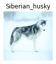
def predict_tftrt(input_saved_model): """Runs prediction on a single image and shows the result. input_saved_model (string): Name of the input model stored in the current dir """ img_path = './data/img0.JPG' # Siberian_husky img = image.load_img(img_path, target_size=(224, 224)) x = image.img_to_array(img) x = np.expand_dims(x, axis=0) x = preprocess_input(x) x = tf.constant(x) saved_model_loaded = tf.saved_model.load(input_saved_model, tags=[tag_constants.SERVING]) signature_keys = list(saved_model_loaded.signatures.keys()) print(signature_keys) infer = saved_model_loaded.signatures['serving_default'] print(infer.structured_outputs) labeling = infer(x) preds = labeling['probs'].numpy() print('{} - Predicted: {}'.format(img_path, decode_predictions(preds, top=3)[0])) plt.subplot(2,2,1) plt.imshow(img); plt.axis('off'); plt.title(decode_predictions(preds, top=3)[0][0][1])予測結果が正しいかを確認します。
predict_tftrt('resnet50_saved_model_TFTRT_FP16')予測結果が
Siberian_huskyと正しく認識されています。['serving_default'] {'probs': TensorSpec(shape=<unknown>, dtype=tf.float32, name='probs')} ./data/img0.JPG - Predicted: [('n02110185', 'Siberian_husky', 0.5543186), ('n02109961', 'Eskimo_dog', 0.41910216), ('n02110063', 'malamute', 0.021393897)]
TF-TRTのFP32と同様のコードでベンチマークを行います。
コードは同様ですがNotebookを再起動したため、再定義します。ベンチマーク結果はTF-TRTのFP32に比べ1.69倍になっています。
def benchmark_tftrt(input_saved_model): saved_model_loaded = tf.saved_model.load(input_saved_model, tags=[tag_constants.SERVING]) infer = saved_model_loaded.signatures['serving_default'] N_warmup_run = 50 N_run = 1000 elapsed_time = [] for i in range(N_warmup_run): labeling = infer(batched_input) for i in range(N_run): start_time = time.time() labeling = infer(batched_input) #prob = labeling['probs'].numpy() end_time = time.time() elapsed_time = np.append(elapsed_time, end_time - start_time) if i % 50 == 0: print('Step {}: {:4.1f}ms'.format(i, (elapsed_time[-50:].mean()) * 1000)) print('Throughput: {:.0f} images/s'.format(N_run * batch_size / elapsed_time.sum()))benchmark_tftrt('resnet50_saved_model_TFTRT_FP16')Throughput: 1233 images/sTF-TRT INT8のモデル
FP16と同様の部分が多いので異なっている部分のみ説明します。
calibration_input_fnでキャリブレーションデータを取得する関数を定義します。
converter.convert(calibration_input_fn=calibration_input_fn)でキャリブレーション処理して活性化関数の閾値を設定します。この関数はyieldで返すgeneratorとして定義する必要があります。以下のドキュメントの”TrtGraphConverter.convert(calibration_input_fn)”にその内容が記述されています。
2.4. TF-TRT API In TensorFlow 2.0
The argument calibration_input_fn is a generator function that yields input data as a list or tuple, which will be used to execute the converted signature for INT8 calibration.print('Converting to TF-TRT INT8...') conversion_params = trt.DEFAULT_TRT_CONVERSION_PARAMS._replace( precision_mode=trt.TrtPrecisionMode.INT8, max_workspace_size_bytes=8000000000, use_calibration=True) converter = trt.TrtGraphConverterV2( input_saved_model_dir='resnet50_saved_model', conversion_params=conversion_params) def calibration_input_fn(): yield (batched_input, ) converter.convert(calibration_input_fn=calibration_input_fn) converter.save(output_saved_model_dir='resnet50_saved_model_TFTRT_INT8') print('Done Converting to TF-TRT INT8')予測処理をして正しく認識できているか確認します。
predict_tftrt('resnet50_saved_model_TFTRT_INT8')下記の結果になっているので正しく認識できていることが分かります。
['serving_default']
{'probs': TensorSpec(shape=<unknown>, dtype=tf.float32, name='probs')}
./data/img0.JPG - Predicted: [('n02110185', 'Siberian_husky', 0.55078125), ('n02109961', 'Eskimo_dog', 0.42236328), ('n02110063', 'malamute', 0.021530151)]
推論性能はTF-TRTのFP16に比べて1.004倍程度の向上にとどまっています。これはINT8がサポートされていないGPUを使用したためです。
benchmark_tftrt('resnet50_saved_model_TFTRT_INT8')Throughput: 1239 images/sGoogle Colaboratory以外での環境構築方法
Google Colaboratoryは予め環境構築がされているため、特定のライブラリの導入が必要がない点やNotebook上の動作が通常とは異なる点、GPUの違いがあるため、他の環境で今回のコードを再現する場合のポイントを記入しました。
下記の内容はNotebook内で記述されていますが、お使いの環境によってはこのうち、dpkgとapt-getにsudo権限などが必要です。その場合、ターミナル等でsudoを付けて実行してください。
%%bash
wget https://developer.download.nvidia.com/compute/machine-learning/repos/ubuntu1804/x86_64/nvidia-machine-learning-repo-ubuntu1804_1.0.0-1_amd64.deb

dpkg -i nvidia-machine-learning-repo-*.deb
apt-get update

sudo apt-get install libnvinfer5
GPU メモリーがP100(16GB)より小さい場合は下記の設定をして、必要な分だけGPUメモリを確保する設定が必要です。
import os
os.environ['TF_FORCE_GPU_ALLOW_GROWTH'] = 'true'
TensorRTの変換時やINT8のキャリブレーションを行う際にGPUメモリが足りなくなる場合は、例えば以下のようにmax_workspace_size_bytesを下げてください。
conversion_params = trt.DEFAULT_TRT_CONVERSION_PARAMS._replace(
    precision_mode=trt.TrtPrecisionMode.INT8,
    # TensorRTが確保するGPUメモリ設定部
    max_workspace_size_bytes=500000000,
    use_calibration=True)
Jetsonでの環境構築
著者が確認した範囲ではJetPack4.3(TensorFlow 2.1.0)とJetPack4.2.2(TensorFlow2.0.0)が動作するため、もし試したい方はJetPack4.3(TensorFlow 2.1.0)もしくはJetPack4.2.2(TensorFlow2.0.0)にしてお試しください。
JetsonでTensorFlowを導入する場合は依存ライブラリの導入が必要なため、下記の資料を参考にインストールすることをお勧めします。
また今回のモデルはResNet50を使用していますがTensorFlow-TensorRT変換に時間を要するため、Jetsonのような限られたリソースの環境であればより小さいモデルであるMobileNetなどで試すことをお勧めします。


- 投稿日:2020-05-27T09:51:17+09:00
tensorflow.python.framework.errors_impl.ResourceExhaustedErrorでOOMが走るときの対処方法
Keras-Yolov3 でGPUを動かしたときにメモリが足りないときの対処方法
YOLOv3 (Tensorflow backend) をGPUを使ってモデルを作成しようとした時にOOMが動いてしまう。
https://github.com/qqwweee/keras-yolo3tensorflow.python.framework.errors_impl.ResourceExhaustedError: OOM when allocating tensor with shape[32,104,104,128] and type float on /job:localhost/replica:0/task:0/device:GPU:0 by allocator GPU_0_bfc
Batchサイズを32 -> 8 に変更したところ、動くようになった。
train.py@@ -54,7 +54,7 @@ def _main(): # use custom yolo_loss Lambda layer. 'yolo_loss': lambda y_true, y_pred: y_pred}) - batch_size = 32 + batch_size = 8 print('Train on {} samples, val on {} samples, with batch size {}.'.format(num_train, num_val, batch_size)) model.fit_generator(data_generator_wrapper(lines[:num_train], batch_size, input_shape, anchors, num_classes), steps_per_epoch=max(1, num_train//batch_size), @@ -73,7 +73,7 @@ def _main(): model.compile(optimizer=Adam(lr=1e-4), loss={'yolo_loss': lambda y_true, y_pred: y_pred}) # recompile to apply the change print('Unfreeze all of the layers.') - batch_size = 32 # note that more GPU memory is required after unfreezing the body + batch_size = 8 # note that more GPU memory is required after unfreezing the body print('Train on {} samples, val on {} samples, with batch size {}.'.format(num_train, num_val, batch_size)) model.fit_generator(data_generator_wrapper(lines[:num_train], batch_size, input_shape, anchors, num_classes), steps_per_epoch=max(1, num_train//batch_size),