20200103のTensorFlowに関する記事は6件です。

投稿日：2020-01-03T22:16:11+09:00

[前処理編] ロイター通信のデータセットを用いて、ニュースをトピックに分類するモデル(MLP)をkerasで作る（TensorFlow 2系）

概要

kerasを使ったテキスト分類を試し、記事にまとめます。
データセットはtensorflowに内蔵されたロイター通信のデータセットです（英語のテキストデータ）。

Keras MLPの文章カテゴリー分類を理解するというブログ記事を参考に、一度取り組んだことがあります。
今回はドキュメントを引きつつ手を動かしており、理解を深める目的でこの記事をアウトプットします。
構築したモデルは、非常にシンプルなMLPです。

分量が長くなったので2つに分けます：

本記事で扱うこと

データセットについて

前処理について

次の記事で扱うこと

モデルの学習について

モデルの性能評価について

動作環境
$ sw_vers
ProductName:    Mac OS X
ProductVersion: 10.14.6
BuildVersion:   18G103
$ python -V  # venvモジュールによる仮想環境を利用
Python 3.7.3
$ pip list  # 主要なものを抜粋
ipython              7.11.0
matplotlib           3.1.2
numpy                1.18.0
pip                  19.3.1
scikit-learn         0.22.1
scipy                1.4.1
tensorflow           2.0.0
データセット

読み込み

tensorflow.keras.datasets.reuters.load_data(ドキュメント)で読み込むことができます。
test_split引数のデフォルト値が0.2のため、学習用8割、テスト用2割に分かれて読み込まれます。
※初回実行時は、データがダウンロードされます。
In [1]: from tensorflow.keras.datasets import reuters

In [2]: (x_train, y_train), (x_test, y_test) = reuters.load_data()

In [3]: len(y_train), len(y_test)
Out[3]: (8982, 2246)  # 合計 11228 件
ラベルを見る

ラベルはニュースのトピックを表すそうです。
試しにラベルを1つ見てみましょう。
In [4]: y_train[1000]
Out[4]: 19
数値で表されています（※それぞれがどんなトピックなのかまでは調べきれていません）。

学習用とテスト用のデータ全体で何種類のラベルがあるか確認します。
numpy.ndarrayのy_trainとy_testをリストに変換して、collections.Counter(ドキュメント)に渡します。
In [5]: from collections import Counter
In [8]: counter = Counter(list(y_train) + list(y_test))

In [9]: len(counter)
Out[9]: 46
全部で46のトピックがありました。

トピックごとに何件あるか確認します。
In [10]: for i in range(46):
    ...:     print(f'{i}: {counter[i]},')
    ...:
0: 67,
1: 537,
2: 94,
3: 3972,
4: 2423,
5: 22,
6: 62,
7: 19,
8: 177,
9: 126,
10: 154,
11: 473,
12: 62,
13: 209,
14: 28,
15: 29,
16: 543,
17: 51,
18: 86,
19: 682,
20: 339,
21: 127,
22: 22,
23: 53,
24: 81,
25: 123,
26: 32,
27: 19,
28: 58,
29: 23,
30: 57,
31: 52,
32: 42,
33: 16,
34: 57,
35: 16,
36: 60,
37: 21,
38: 22,
39: 29,
40: 46,
41: 38,
42: 16,
43: 27,
44: 17,
45: 19,
3と4のトピックが図抜けて多く、約57%を占めます。
トピックに含まれる記事の数に偏りがありますが、今回は46クラスへの分類という問題設定で進めます。

ニュースのテキストを見る

ニュースも1つ見てみましょう。
In [12]: x_train[1000]
Out[12]:
[1,
 437,
 495,
 1237,
 55,
 9070,
 :
 12]
整数からなるリストが表示されました。
今回のデータセットの場合、単語が数値に変換されています。
元のテキストを確認してみます。

まず、単語と数値の対応表は、tensorflow.keras.datasets.reuters.get_word_index(ドキュメント)で取得できます。
※初回実行時は、データがダウンロードされます。
In [16]: word_index = reuters.get_word_index()

In [17]: len(word_index)
Out[17]: 30979

In [18]: word_index
Out[18]:
{'mdbl': 10996,
 'fawc': 16260,
 'degussa': 12089,
 'woods': 8803,
 'hanging': 13796,
 'localized': 20672,
 :
 'hebei': 9407,
 ...}

In [19]: for word, index in word_index.items():
    ...:     if index in [0, 1, 2]:
    ...:         print(word, index)
    ...:
the 1
of 2

In [20]: for word, index in word_index.items():
    ...:     if index in [30978, 30979, 30980]:
    ...:         print(word, index)
    ...:
jung 30978
northerly 30979
word_indexは単語に対する数値の辞書です。
この対応を逆にして数値に対する単語の辞書を用意すればよさそうです。
ここで、x_trainとx_testに使われた整数は、word_indexの整数とずれていることに対応する必要があります。

ずれる理由は load_dataの3つの引数にあります。

1. 開始を表す数値：start_char=1

The start of a sequence will be marked with this character. Set to 1 because 0 is usually the padding character.

x_trainとx_testの中で1は開始を表します。
0がpadding character（埋め草文字。余白を埋めるための文字）に使われるため、1がデフォルト値となっているそうです。

2. 対応しない語を表す数値：oov_char=2

words that were cut out because of the num_words or skip_top limit will be replaced with this character.

num_wordsやskip_top引数によって、使う単語の範囲を区切ることで、対応しない語がoov_charに置き換えられます。
今のx_trainやx_testを取得する際、これらの引数を指定していないため、oov_charは現時点では無関係です。
（load_dataのドキュメントを見ると、oovはout of vocabularyの略のようです）

3. 単語に対応する数値の最初の値：index_from=3

index actual words with this index and higher.

数値のうち、0, 1, 2が意味を持っているため、単語の対応がずれるわけです。
index_from引数によりx_trainやx_testはword_indexの0が3に該当するという対応¹で読み込まれています。

ニュースを単語の並びとして見るために、数値のズレを考慮して、数値: 単語という辞書を作ります。
In [22]: index_word_map = {
    ...:     index + 3: word for word, index in word_index.items()
    ...: }
    ...: index_word_map[0] = "[padding]"
    ...: index_word_map[1] = "[start]"
    ...: index_word_map[2] = "[oov]"
In [23]: len(index_word_map)
Out[23]: 30982
この辞書を使うことでx_train, x_testの整数の並びから文章を復元することができました。
In [24]: for index in x_train[1000]:
    ...:     print(index_word_map[index], end = " ")
    ...:
[start] german banking authorities are weighing rules for banks' off balance sheet activities in an attempt to cope with the growing volume of sophisticated capital market instruments banking sources said interest rate and currency swaps and ...
前処理

テキストの前処理

整数で表されたニュース記事の長さはまちまちです。
In [31]: for x in x_train[998:1003]:
    ...:     print(len(x))
    ...:
133
51
626
17
442
そこで長さが揃うように変換して前処理します。
今回は、各ニュース記事を、ニュース記事全体に登場する頻度の上位1000語が含まれるか否かで表します。

例えば、上位1000語の中に「currency」という単語があり、対応する整数は500とします。
各記事を0か1の並びで表すとき、currencyという語を含む記事は、インデックス500に1が来ます。
currencyという語を含まない記事は、インデックス500が0です。
これが他の語にも当てはまります。

この変換により、

ニュース記事の長さが1000に揃います

ニュース記事は1000個の0または1の並びで表されます

load_dataメソッドのnum_words引数²に1000を渡して、登場する頻度の上位1000語でx_train, x_testを表すように変換します。
In [32]: (x_train, y_train), (x_test, y_test) = reuters.load_data(num_words=1000)
    ...:

In [33]: len(y_train), len(y_test)
Out[33]: (8982, 2246)
num_wordsを登場頻度の上位1000語としたので、そこに含まれない語はoov_char(整数では2)としてx_train, x_testで表されます。
In [34]: for index in x_train[1000]:
    ...:     print(index_word_map[index], end = " ")
    ...:
[start] german banking [oov] are [oov] [oov] for [oov] off balance [oov] [oov] in an [oov] to [oov] with the growing volume of [oov] capital market [oov] banking sources said interest rate and currency [oov] and ...
この段階ではニュース記事の長さはまだ揃っていません。
上位1000語がニュース記事に含まれるか否かを表すために、tensorflow.keras.preprocessing.text.Tokenizer(ドキュメント)を使います。

Tokenizerの初期化でnum_words引数に1000を渡します。
Tokenizerを使った処理でnum_words-1の語が考慮されます。

num_words: the maximum number of words to keep, based
on word frequency. Only the most common num_words-1 words will
be kept.
In [37]: from tensorflow.keras.preprocessing.text import Tokenizer

In [42]: tokenizer = Tokenizer(1000)
load_dataで上位1000語を取り出しているので、x_train, x_testに含まれる整数の最大は999です³。
In [71]: max_index = 0

In [72]: for x in list(x_train)+list(x_test):
    ...:     now_max = max(x)
    ...:     if now_max > max_index:
    ...:         max_index = now_max
    ...:

In [73]: max_index
Out[73]: 999
sequences_to_matrixメソッド(ドキュメント)で、x_train, x_testをそれぞれ変換します。
In [36]: x_train.shape, x_test.shape
Out[36]: ((8982,), (2246,))

In [76]: x_train = tokenizer.sequences_to_matrix(x_train, "binary")

In [77]: x_test = tokenizer.sequences_to_matrix(x_test, "binary")

In [78]: x_train.shape, x_test.shape
Out[78]: ((8982, 1000), (2246, 1000))
全てのニュース記事が長さが1000で表されました。

sequences_to_matrixのドキュメントによると、

a sequence is a list of integer word indices

すなわち、sequenceとは「単語を表す整数のリスト（意訳）」なので、x_train, x_testはまさしくsequenceです。

第2引数の指定ですが、"binany"の場合は各語が存在するかしないかの0/1で表されます。
他に、"count", "tfidf", "freq"を指定できるそうです。

変換されたニュース記事を試しに1つ見てみると
In [58]: x_train[1000]
Out[58]:
array([0., 1., 1., 0., 1., 1., 1., 1., 1., 1., 1., 0., 1., 1., 0., 0., 1.,
       ...
と0/1で表現されています。
index_word_mapの中で0（埋め草文字にあたる）や、3（もともと0の語がないので、3というキーがない）はどのニュースにも登場しないので0です。
1([start])や2([oov])、4(the)、5(of)などはx_train[1000]に登場するので1となっています。

テキストの前処理は以上です。

ラベルの前処理

ラベル（ニュースのトピック）は0〜45のいずれかですが、これをone-hot表現に変換します。
（one-hot表現とする理由は、ラベル同士に大小関係を持たせないようにするため）

tensorflow.keras.utils.to_categorical(ドキュメント)を使います。
In [80]: y_train.shape, y_test.shape
Out[80]: ((8982,), (2246,))

In [81]: from tensorflow import keras

In [85]: number_of_classes = len(counter)

In [86]: y_train = keras.utils.to_categorical(y_train, number_of_classes)

In [88]: y_test = keras.utils.to_categorical(y_test, number_of_classes)

In [89]: y_train.shape, y_test.shape
Out[89]: ((8982, 46), (2246, 46))
ラベルをインデックスと見立てて、ラベルのインデックスだけ1、他は0という形式に変換されます。
y_train[1000]は19でしたが、y_train[1000][19]が1、他は0となるように変換されています。
In [90]: y_train[1000]
Out[90]:
array([0., 0., 0., 0., 0., 0., 0., 0., 0., 0., 0., 0., 0., 0., 0., 0., 0.,
       0., 0., 1., 0., 0., 0., 0., 0., 0., 0., 0., 0., 0., 0., 0., 0., 0.,
       0., 0., 0., 0., 0., 0., 0., 0., 0., 0., 0., 0.], dtype=float32)
前処理は以上です。

本記事のまとめ

データセットについて

ロイター通信のニュースのトピック分類データ（多クラス分類）

ラベルは46クラスあり、含まれるニュースの件数に偏りがある

ニュースは整数のリストで表されている。単語の並びへ復元して元のニュースを確認できる

前処理について

テキストを固定長の0/1の並びに変換（登場頻度上位1000語のそれぞれが含まれるか否か）

ラベルをone-hot表現に変換

本記事は[モデル構築編]（近日公開）に続きます。

word_indexは0というキーを持ちませんが、1は4、2は5、、、のように対応するということです ↩

「max number of words to include. Words are ranked by how often they occur (in the training set) and only the most frequent words are kept」（学習用データの中で頻出する上位何語を使って、x_train, x_testとして取り出すかの指定です） ↩

index_word_mapでキーが999までの単語ということです ↩

　 Tweet
Qiitaで続きを読む

投稿日：2020-01-03T17:28:09+09:00

DeepLearningでアボカドの硬さ推定[番外編1]

DeepLearningでアボカドの硬さを推定する話（番外編）

DeepLearningでアボカドの硬さ推定[0]では音声データからアボカドの硬さを推定する内容を投稿しました。
今回は本編のついでに撮影していた画像データを分析する番外編です。

アボカドからデータ収集

使ったデバイス

・iPhone6s （画像データ）
・貫入硬度計（硬度データ）
貫入硬度計による教師データはDeepLearningでアボカドの硬さ推定[0]の使いまわしになります。

画像からRGB取得

オープンソースの画像処理ソフトImageJを用いました。
手作業にて果実の輪郭を選択し、1果実につき1つの平均RGB値を取得してCSVに書き出します。

分析

前処理

ImageJから取得したRGBデータの各色を三色合計値で割り、RGBを比の形にしました。

結果

相関係数（Excelにて計算）

赤色と硬度：R=-0.79
緑色と硬度：R=0.85
青色と硬度：R=0.07
赤と緑に強い相関関係が認められました。
まあ未熟なアボカドは緑色をしているし、
熟すにつれて赤色っぽくなっていくのは肉眼でも観察できます。
妥当なところかもしれません。

重回帰

赤と緑と硬度で回帰分析を行いました。
決定係数は0.75とまあまあの精度。

今回はここまでです。
次回番外編2ではTestR2を計算してみます。
はたして、スマホのカメラはアボカドの硬度予測センサとして使い物になるのでしょうか。
こうご期待。

　 Tweet
Qiitaで続きを読む

投稿日：2020-01-03T16:03:30+09:00

TensorFlow2 + Keras による画像分類に挑戦8 ～最適化アルゴリズムと損失関数を選択する～

はじめに

TensorFlow2 + Keras を利用した画像分類（Google Colaboratory 環境）についての勉強メモ（第8弾）です。題材は、ド定番である手書き数字画像（MNIST）の分類です。

TensorFlow2 + Keras による画像分類に挑戦シリーズ

1. とりあえず動かす

2. 入力データを詳しくみてみる

3. MNISTデータを可視化してみる

4. 学習済みモデルで予測させてみる

5. 分類に失敗する画像を観察してみる

6. 自分で用意した画像の前処理・分類をしてみる

7. 層タイプ・活性化関数について理解する

8. 最適化アルゴリズムと損失関数を選択する

9. モデルの学習、セーブ＆ロードをしてみる

前回は、TF公式HPの「初心者のための TensorFlow 2.0 入門」で取り上げられているニューラルネットワークモデルについて、それを構成する各層（Dense層、Dropout層、Flatten層）と活性化関数（ReLU関数、Softmax関数）の観点から、その概要を理解しました。

今回は、チュートリアルのプログラムの model.compile のところ（最適化アルゴリズムや損失関数の設定）について、理解していきたいと思います。
model.compile(optimizer='adam',
              loss='sparse_categorical_crossentropy',
              metrics=['accuracy'])
また、同じ構成のニューラルネットモデルであっても、学習に用いる最適化アルゴリズムの違いにより正解率（accuracy）や損失関数値（loss）、収束速度、計算時間が大きく変わることを実験により確認します。そこでは、次のようなグラフを作成していきます。

モデルのコンパイル model.compile(...) について

TF公式HPの「初心者のための TensorFlow 2.0 入門」のチュートリアルプログラムのでは、tf.keras.models.Sequential(...) によって、ニューラルネットの層構成を定義したあと、それをトレーニングする前に、compile(optimizer=..., loss=..., metrics=...) というプロセスをはさんでいます。

model.compile() のリファレンスはこちらを参照

このプロセスでは、ニューラルネットモデルのトレーニング（重みパラメータの最適化）で、評価指標として使用する損失関数（誤差関数、目的関数、Loss Function）の設定や、最適化アルゴリズム（勾配法、Optimizer）の設定しています。

また、metrics は、トレーニングのログとして誤差関数（loss）以外に出力する項目を指示するもので、トレーニングそのものに何らかの影響を与える設定ではないようです（いまいち自信なし）。

以下、これらについて詳しく見ていきます。

最適化アルゴリズム（Optimizer）の選択

compile の optimizer= 引数では、トレーニングに使用する最適化アルゴリズム（勾配法、Optimizer）を選択します。ここで、選択可能な Optimizer は、こちらのリファレンスから一覧をみることができます。

2020/01/03 の時点では、次の Optimizer が利用できます。なお、「深層学習の最適化アルゴリズム」を参考にアルゴリズムが発表された年も併記しています。

SGD

Ftrl

Adagrad：2011年

RMSprop：2012年

Adadelta：2012年

Adam：2014年

Adamax：2015年

Nadam：2016年

上記の xxx を使って optimizer='xxxx' のように文字列で指定することも、optimizer=tf.optimizers.Adam() のように指定して与えることも可能です（両者で微妙に大文字小文字が違ったりするので注意、詳細はリファレンスで確認）。

チュートリアルでも採用されているように、まずは Adam から試してみるのがよいのかもしれません。無論、扱う問題やNNモデルの構造や規模により、最適な Optimizer は変わるので、より良いトレーニングをさせるためには、色々と手法を変えて試すことが要求されます。

あとで、MNISTについて、最適化アルゴリズムを変えてトレーニングする実験を行ないます。

損失関数（loss）の選択

深層学習におけるトレーニングとは、最適化問題の求解と同義です。最適化問題で言うところの目的関数が「損失関数（最小化）」、決定変数が「ニューラルネットのパラメータ（重みやバイアス）」になります。

損失関数は、「NNモデルによる予測値」と「正解値」を入力として、その差異・乖離度を定量化して出力する関数です。トレーニングでは、この損失関数の出力値を最小化するようにパラメータ（重みやバイアス）の調整が進みます。

MNISTのような多クラス分類問題では、通常、その損失関数として「交差エントロピー誤差（Cross Entropy Error）」という尺度を計算するものが使われます。よって、チュートリアルでも loss='sparse_categorical_crossentropy' のように交差エントロピー誤差を計算するように設定されています。なお、選択可能な損失関数は、こちらから一覧を見ることができます。

なお、交差エントロピー誤差の計算に関しては、sparse_categorical_crossentropy と categorical_crossentropy の2つがありますが、違いは以下の通りです。

sparse_categorical_crossentropy は、MNISTのように多クラス分類問題の正解データ（ラベル）をカテゴリ番号で与えている場合に使います。正解が「0」「4」「2」のとき、[2,7,5] のように与えている場合。

categorical_crossentropy は、多クラス分類問題の正解データ（ラベル）を、one-hot表現（one-hotベクトル）で与えている場合に使います。正解が「0」「4」「2」のとき、[[1,0,0,0,0,0,0,0,0,0],[0,0,0,0,1,0,0,0,0,0],[0,0,1,0,0,0,0,0,0,0]] のように与えている場合。

仮に、カテゴリが4個だったとして、正解データが $[0,1,0,0]$、予測データが $[0.1,0.6,0.2,0.1]$ だったとすれば、交差エントロピー誤差 $\mathrm{CE}$ は次のように計算できます。
\begin{align}
\mathrm{CE} &= - ( 0\times \log_{\,e} 0.1 + 1\times \log_{\,e} 0.6 + 0\times \log_{\,e} 0.2 + 0\times \log_{\,e} 0.1  ) \\
& = -\log_{\,e} 0.6 \\
& = 0.51083
\end{align}
テストデータが複数ある場合は、平均をとればOKです。ところで、正解データは、$0$ または $1$ に限られるので、複数のテストデータ（$1,2,\cdots,n$）の平均交差エントロピー誤差は、シンプルに次のように計算できます。

$$ \mathrm{CE} = -\frac{1}{n} \sum_{i=1}^{n} \log_{\ e} p_{i} $$

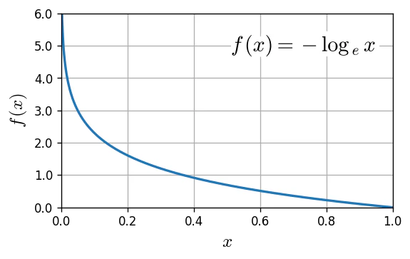
なお、$f(x) = - \log_{\ e} x $ について、$0.0 < x \le 1.0$ でプロットすると、次のようになります。

正解データと予測データが一致していれば、$-\log_{\ e}1.0=0.0$ で、CE誤差はゼロとなります。なお、$\log_{\ e}0.0=-\infty $ なのでプログラムで計算する際には工夫が必要です。

手動で交差エントロピー誤差（loss）を計算

チュートリアルのプログラムを実行すると、model.evaluate(x_test, y_test, verbose=2) のログとして次のように loss を出力してくれます。

10000/10000 - 0s - loss: 0.0734 - accuracy: 0.9775

これを自分で計算してみます。
交差エントロピー誤差を計算
import numpy as np
import math

s_test = model.predict(x_test) # 学習済みモデルで予測

# 交差エントロピー誤差（Cross Entropy Error）
ce = 0
n = len(y_test)
for i in range(0,n) :
  ce = ce - math.log(s_test[i,y_test[i]])
ce = ce/n
print(f'CE(手計算) = {ce} ')
実行結果は以下のようになりました。

CE(手計算) = 0.07341307844041595

これは、evaluate(...) で出力された loss: 0.0734 に一致します。

最適化アルゴリズムを変えて学習、結果の比較

現時点で、TF+Keras で選択可能な8つの最適化アルゴリズム（SGD、Ftrl、Adagrad、RMSprop、Adadelta、Adam、Adamax、Nadam）で、MNISTをターゲット学習、評価を行ないました。

Epochs数=100 として、トレーニングプロセスのEpoch毎に、トレーニングデータ x_train に対する正答率（accuracy）と損失関数値（loss）、テストデータ x_test に対する正答率（val_accuracy）と損失関数値（val_loss）を取得してプロットしました。

先に結果を表示します。

正答率（accuracy）

Y軸の範囲を拡大します。

汎化性能を考慮したテストデータに対する結果として、AdaMax(2015) が非常に優れています。SGDは、非常に時間がかかりますが、最終的には AdaMax(2015) と同じ程度の正答率が得らるモデルになっています。

損失関数値（loss）

Y軸の範囲を拡大します。

RMSprop(2012)では、過学習を起していることが確認できます。最終的には SGD が最も優れたスコアになっています。

計算時間

Google Colab.環境で実行したとき、Epochs=100 に要した時間です。

（最適化手法については、完全にブラックボックスとして扱っているので下手なことは言えませんが・・・）どうも「AdaMax」が良さそうです。

プログラム

上記のグラフを求めるために使ったプログラムです。
データの計算と取得
import time
import pickle
import tensorflow as tf

tf.keras.backend.clear_session()  # セッションクリア

# (1) データセットの準備
mnist = tf.keras.datasets.mnist
(x_train, y_train), (x_test, y_test) = mnist.load_data()
x_train, x_test = x_train / 255.0, x_test / 255.0

# (2) NNモデルの構築
model = tf.keras.models.Sequential()
model.add( tf.keras.layers.Flatten(input_shape=(28, 28)) )
model.add( tf.keras.layers.Dense(128, activation=tf.nn.relu) )
model.add( tf.keras.layers.Dropout(0.2) )
model.add( tf.keras.layers.Dense(10, activation=tf.nn.softmax) )

# (3) NNモデルの学習設定・学習・評価
epochs = 100
prm = [ dict(label='SGD',            optm='SGD')     ,
        dict(label='FTRL',           optm='Ftrl')    ,
        dict(label='AdaGrad(2012)',  optm='Adagrad') ,
        dict(label='RMSprop(2012)',  optm='RMSprop') ,
        dict(label='AdaDelta(2012)', optm='Adadelta'),
        dict(label='Adam(2014)',     optm='Adam')    ,
        dict(label='AdaMax(2015)',   optm='Adamax')  , 
        dict(label='NAdam(2016)',    optm='Nadam')    ]

for p in prm :
  print(f"■ 最適化アルゴリズム {p['label']}")
  t = time.time() 
  model.compile(optimizer=p['optm'],
                loss='sparse_categorical_crossentropy',
                metrics=['accuracy'])
  h = model.fit(x_train, y_train, 
                validation_data=(x_test,y_test), 
                epochs=epochs)
  p['log'] = h.history
  p['time'] = time.time() - t
  p['epochs'] = epochs

results = prm

# 結果の保存
path = 'optimizer-1.pickle'
with open(path,mode='wb') as f :
  pickle.dump(results,f)
データの可視化
import numpy as np
import matplotlib.pyplot as plt

title = dict( )
title['accuracy'] = 'Accuracy (TarinData)'
title['val_accuracy'] = 'Accuracy (TestData)'
title['loss'] = 'Loss (TarinData)'
title['val_loss'] = 'Loss (TestData)'

# 正答率
fig, ax = plt.subplots(nrows=1, ncols=2, sharey='row', figsize=(10,3), dpi=120)
plt.subplots_adjust(wspace=0.03)
for i, v in enumerate(['accuracy','val_accuracy']) :
  for r in results :
    ax[i].plot( range(1,r['epochs']+1),r['log'][v],label=r['label'])
    ax[i].set_xlim(1,r['epochs'])
    ax[i].set_ylim( 0.97,1.00 ) # ■■■要調整■■■
    ax[i].set_title( title[v] )
    ax[i].tick_params(which='both', direction='in')
    ax[i].grid(True)
  ax[1].legend(bbox_to_anchor=(1.02, 1), loc='upper left', borderaxespad=0)
plt.show()

# 損失関数値
fig, ax = plt.subplots(nrows=1, ncols=2, sharey='row', figsize=(10,3), dpi=120)
plt.subplots_adjust(wspace=0.03)
for i, v in enumerate(['loss','val_loss']) :
  for r in results :
    ax[i].plot( range(1,r['epochs']+1),r['log'][v],label=r['label'])
    ax[i].set_xlim(1,r['epochs'])
    ax[i].set_ylim( 0.0, 0.3 ) # ■■■要調整■■■
    ax[i].set_title( title[v] )
    ax[i].tick_params(which='both', direction='in')
    ax[i].grid(True)
  ax[1].legend(bbox_to_anchor=(1.02, 1), loc='upper left', borderaxespad=0)
plt.show()

# 時間
labels = list()
times = list()
for r in results :
  labels.append(r['label'])
  times.append(r['time'])

plt.figure(dpi=120,figsize=(6,3))
plt.bar(labels,times)
plt.ylabel('Time (sec)')
plt.xticks(rotation=-90)
plt.gca().set_axisbelow(True)
plt.grid(axis='y')
plt.show()
次回

次回は、モデルの学習 model.fit(...) の引数（エポック数、バッチ数、バリデーション用データ設定など）について、取り上げます。また、学習済みモデルのファイルセーブとロードについても扱っていきたいと思います。

おまけ

交差エントロピー誤差で使う $-\log_{\,e} x$ のグラフを描くためのプログラムです。
-log_xのグラフ作成
import numpy as np
import matplotlib.pyplot as plt
import matplotlib.ticker as tk
import matplotlib.patheffects as pe

plt.rcParams['mathtext.fontset'] = 'cm' # 数式用フォント

yt_style = lambda x, pos=None : f'{x:.1f}'

x = np.linspace(0.001, 1, 1000)
y = -np.log(x)
plt.figure(dpi=120,figsize=(5,3))
plt.plot(x,y,lw=2)
plt.xlim(0,1)
plt.ylim(0,6)
plt.gca().yaxis.set_major_formatter(tk.FuncFormatter(yt_style))
plt.xlabel('$x$',fontsize=15)
plt.grid()
plt.ylabel('$f\,(x)$',fontsize=15)
t = plt.text(0.95,5, r'$f\,(x)=-\log_{\,e}\,x$', fontsize=18,
         ha='right',va='center')
t.set_path_effects([pe.Stroke(linewidth=9, foreground='white'), pe.Normal()])

　 Tweet
Qiitaで続きを読む

投稿日：2020-01-03T14:03:52+09:00

質問です。rasｐberry pi 3 modelB にprotocolbuffersをmakeできない。

ラズベリーパイで画像認識をするために、Qiitaの投稿などをもとに”protocolbuffers”をインストールしています。” ./configure”でエラーが出てしまいます。その後"make”しようとしていますが、”make: *** ターゲットが指定されておらず, makefile も見つかりません. 中止.”となり、前に進むことが出来ません。
どなたか、解決方法を教えて頂けないでしょうか？
投稿元：https://qiita.com/kobayuta/items/59c7b84caf8994071357

以下エラーコード：
$ cd protobuf-3.7.1
$ ./configure
checking whether to enable maintainer-specific portions of Makefiles... yes
checking build system type... armv7l-unknown-linux-gnueabihf
checking host system type... armv7l-unknown-linux-gnueabihf
checking target system type... armv7l-unknown-linux-gnueabihf
checking for a BSD-compatible install... /usr/bin/install -c
checking whether build environment is sane... yes
checking for a thread-safe mkdir -p... /bin/mkdir -p
checking for gawk... no
checking for mawk... mawk
checking whether make sets $(MAKE)... yes
checking whether make supports nested variables... yes
checking whether UID '1000' is supported by ustar format... yes
checking whether GID '1000' is supported by ustar format... yes
checking how to create a ustar tar archive... gnutar
checking for gcc... no
checking for cc... no
checking for cl.exe... no
configure: error: in /home/pi/protobuf-3.7.1': configure: error: no acceptable C compiler found in $PATH Seeconfig.log' for more details
$ make
make: *** ターゲットが指定されておらず, makefile も見つかりません. 中止.
$

　 Tweet
Qiitaで続きを読む

投稿日：2020-01-03T14:03:52+09:00

質問です。rasberry pi 3 model3 にprotocolbuffersをmakeできない。

ラズベリーパイで画像認識をするために、Qiitaの投稿などをもとに”protocolbuffers”をインストールしています。” ./configure”でエラーが出てしまいます。その後"make”しようとしていますが、”make: *** ターゲットが指定されておらず, makefile も見つかりません. 中止.”となり、前に進むことが出来ません。
どなたか、解決方法を教えて頂けないでしょうか？
投稿元：https://qiita.com/kobayuta/items/59c7b84caf8994071357

以下エラーコード：
$ cd protobuf-3.7.1
$ ./configure
checking whether to enable maintainer-specific portions of Makefiles... yes
checking build system type... armv7l-unknown-linux-gnueabihf
checking host system type... armv7l-unknown-linux-gnueabihf
checking target system type... armv7l-unknown-linux-gnueabihf
checking for a BSD-compatible install... /usr/bin/install -c
checking whether build environment is sane... yes
checking for a thread-safe mkdir -p... /bin/mkdir -p
checking for gawk... no
checking for mawk... mawk
checking whether make sets $(MAKE)... yes
checking whether make supports nested variables... yes
checking whether UID '1000' is supported by ustar format... yes
checking whether GID '1000' is supported by ustar format... yes
checking how to create a ustar tar archive... gnutar
checking for gcc... no
checking for cc... no
checking for cl.exe... no
configure: error: in /home/pi/protobuf-3.7.1': configure: error: no acceptable C compiler found in $PATH Seeconfig.log' for more details
$ make
make: *** ターゲットが指定されておらず, makefile も見つかりません. 中止.
$

　 Tweet
Qiitaで続きを読む

投稿日：2020-01-03T14:03:52+09:00

質問です。rasberry pi 3 modelB にprotocolbuffersをmakeできない。

ラズベリーパイで画像認識をするために、Qiitaの投稿などをもとに”protocolbuffers”をインストールしています。” ./configure”でエラーが出てしまいます。その後"make”しようとしていますが、”make: *** ターゲットが指定されておらず, makefile も見つかりません. 中止.”となり、前に進むことが出来ません。
どなたか、解決方法を教えて頂けないでしょうか？
投稿元：https://qiita.com/kobayuta/items/59c7b84caf8994071357

以下エラーコード：
$ cd protobuf-3.7.1
$ ./configure
checking whether to enable maintainer-specific portions of Makefiles... yes
checking build system type... armv7l-unknown-linux-gnueabihf
checking host system type... armv7l-unknown-linux-gnueabihf
checking target system type... armv7l-unknown-linux-gnueabihf
checking for a BSD-compatible install... /usr/bin/install -c
checking whether build environment is sane... yes
checking for a thread-safe mkdir -p... /bin/mkdir -p
checking for gawk... no
checking for mawk... mawk
checking whether make sets $(MAKE)... yes
checking whether make supports nested variables... yes
checking whether UID '1000' is supported by ustar format... yes
checking whether GID '1000' is supported by ustar format... yes
checking how to create a ustar tar archive... gnutar
checking for gcc... no
checking for cc... no
checking for cl.exe... no
configure: error: in /home/pi/protobuf-3.7.1': configure: error: no acceptable C compiler found in $PATH Seeconfig.log' for more details
$ make
make: *** ターゲットが指定されておらず, makefile も見つかりません. 中止.
$

　 Tweet
Qiitaで続きを読む

20200103のTensorFlowに関する記事は6件です。

[前処理編] ロイター通信のデータセットを用いて、ニュースをトピックに分類するモデル(MLP)をkerasで作る（TensorFlow 2系）

概要

動作環境

データセット

読み込み

ラベルを見る

ニュースのテキストを見る

前処理

テキストの前処理

ラベルの前処理

本記事のまとめ

DeepLearningでアボカドの硬さ推定[番外編1]

DeepLearningでアボカドの硬さを推定する話（番外編）

アボカドからデータ収集

使ったデバイス

画像からRGB取得

分析

前処理

結果

相関係数（Excelにて計算）

重回帰

TensorFlow2 + Keras による画像分類に挑戦8 ～最適化アルゴリズムと損失関数を選択する～

はじめに

モデルのコンパイル `model.compile(...)` について

最適化アルゴリズム（Optimizer）の選択

損失関数（loss）の選択

手動で交差エントロピー誤差（loss）を計算

最適化アルゴリズムを変えて学習、結果の比較

正答率（accuracy）

損失関数値（loss）

計算時間

プログラム

次回

おまけ

質問です。rasｐberry pi 3 modelB にprotocolbuffersをmakeできない。

質問です。rasberry pi 3 model3 にprotocolbuffersをmakeできない。

質問です。rasberry pi 3 modelB にprotocolbuffersをmakeできない。

日付別

タグ一覧

20200103のTensorFlowに関する記事は6件です。

[前処理編] ロイター通信のデータセットを用いて、ニュースをトピックに分類するモデル(MLP)をkerasで作る（TensorFlow 2系）

概要

動作環境

データセット

読み込み

ラベルを見る

ニュースのテキストを見る

前処理

テキストの前処理

ラベルの前処理

本記事のまとめ

DeepLearningでアボカドの硬さ推定[番外編1]

DeepLearningでアボカドの硬さを推定する話（番外編）

アボカドからデータ収集

使ったデバイス

画像からRGB取得

分析

前処理

結果

相関係数（Excelにて計算）

重回帰

TensorFlow2 + Keras による画像分類に挑戦8 ～最適化アルゴリズムと損失関数を選択する～

はじめに

モデルのコンパイル model.compile(...) について

最適化アルゴリズム（Optimizer）の選択

損失関数（loss）の選択

手動で交差エントロピー誤差（loss）を計算

最適化アルゴリズムを変えて学習、結果の比較

正答率（accuracy）

損失関数値（loss）

計算時間

プログラム

次回

おまけ

質問です。rasｐberry pi 3 modelB にprotocolbuffersをmakeできない。

質問です。rasberry pi 3 model3 にprotocolbuffersをmakeできない。

質問です。rasberry pi 3 modelB にprotocolbuffersをmakeできない。

日付別

タグ一覧

モデルのコンパイル `model.compile(...)` について