- 投稿日:2019-05-30T23:47:31+09:00
多層パーセプトロン [TensorFlow2.0でDeep Learning 4]
(目次はこちら)
はじめに
畳み込みニューラルネット Part1 [TensorFlowでDeep Learning 4]をtensorflow2.0で実現するためにはどうしたらいいのかを書く(
tf.keras)。コード
Python: 3.6.8, Tensorflow: 2.0.0a0で動作確認済み
畳み込みニューラルネット Part1 [TensorFlowでDeep Learning 4]
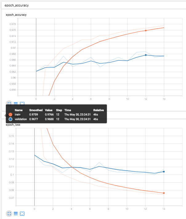
(mnist_fixed_cnn_simple.py)を書き換えると、v2/mnist_fixed_cnn_simple.pyfrom helper import * IMAGE_WIDTH, IMAGE_HEIGHT = 28, 28 CATEGORY_NUM = 10 LEARNING_RATE = 0.1 FILTER_NUM = 2 EPOCHS = 15 BATCH_SIZE = 100 LOG_DIR = 'log_fixed_cnn' class Prewitt(tf.keras.layers.Layer): def build(self, input_shape): v = np.array([[ 1, 0, -1]] * 3) h = v.swapaxes(0, 1) self.kernel = tf.constant(np.dstack([v, h]).reshape((3, 3, 1, 2)), dtype = tf.float32, name='prewitt') self.built = True def call(self, x): x_ = tf.reshape(x, [-1, x.shape[1], x.shape[2], 1]) return tf.abs(tf.nn.conv2d(x_, self.kernel, strides=[1, 1, 1, 1], padding='SAME')) if __name__ == '__main__': (X_train, y_train), (X_test, y_test) = mnist_samples() model = tf.keras.models.Sequential() model.add(Prewitt((IMAGE_HEIGHT * IMAGE_WIDTH, FILTER_NUM), input_shape=(IMAGE_HEIGHT, IMAGE_WIDTH))) model.add(tf.keras.layers.Flatten()) model.add(tf.keras.layers.Dense(CATEGORY_NUM, activation='softmax')) model.compile( loss='categorical_crossentropy', optimizer=tf.keras.optimizers.SGD(LEARNING_RATE), metrics=['accuracy']) cb = [tf.keras.callbacks.TensorBoard(log_dir=LOG_DIR)] model.fit(X_train, y_train, batch_size=BATCH_SIZE, epochs=EPOCHS, callbacks=cb, validation_data=(X_test, y_test)) print(model.evaluate(X_test, y_test))と書ける。ただ、Prewittフィルタの表現が適切かどうかが不安が残るが、動作は適切。
めでたしめでたし。(1epochで、すでに精度高い)
- 投稿日:2019-05-30T23:47:31+09:00
畳み込みニューラルネット Part1 [TensorFlow2.0でDeep Learning 4]
(目次はこちら)
はじめに
畳み込みニューラルネット Part1 [TensorFlowでDeep Learning 4]をtensorflow2.0で実現するためにはどうしたらいいのかを書く(
tf.keras)。コード
Python: 3.6.8, Tensorflow: 2.0.0a0で動作確認済み
畳み込みニューラルネット Part1 [TensorFlowでDeep Learning 4]
(mnist_fixed_cnn_simple.py)を書き換えると、v2/mnist_fixed_cnn_simple.pyfrom helper import * IMAGE_WIDTH, IMAGE_HEIGHT = 28, 28 CATEGORY_NUM = 10 LEARNING_RATE = 0.1 FILTER_NUM = 2 EPOCHS = 15 BATCH_SIZE = 100 LOG_DIR = 'log_fixed_cnn' class Prewitt(tf.keras.layers.Layer): def build(self, input_shape): v = np.array([[ 1, 0, -1]] * 3) h = v.swapaxes(0, 1) self.kernel = tf.constant(np.dstack([v, h]).reshape((3, 3, 1, 2)), dtype = tf.float32, name='prewitt') self.built = True def call(self, x): x_ = tf.reshape(x, [-1, x.shape[1], x.shape[2], 1]) return tf.abs(tf.nn.conv2d(x_, self.kernel, strides=[1, 1, 1, 1], padding='SAME')) if __name__ == '__main__': (X_train, y_train), (X_test, y_test) = mnist_samples() model = tf.keras.models.Sequential() model.add(Prewitt((IMAGE_HEIGHT * IMAGE_WIDTH, FILTER_NUM), input_shape=(IMAGE_HEIGHT, IMAGE_WIDTH))) model.add(tf.keras.layers.Flatten()) model.add(tf.keras.layers.Dense(CATEGORY_NUM, activation='softmax')) model.compile( loss='categorical_crossentropy', optimizer=tf.keras.optimizers.SGD(LEARNING_RATE), metrics=['accuracy']) cb = [tf.keras.callbacks.TensorBoard(log_dir=LOG_DIR)] model.fit(X_train, y_train, batch_size=BATCH_SIZE, epochs=EPOCHS, callbacks=cb, validation_data=(X_test, y_test)) print(model.evaluate(X_test, y_test))と書ける。ただ、Prewittフィルタの表現が適切かどうかが不安が残るが、動作は適切。
めでたしめでたし。(1epochで、すでに精度高い)
- 投稿日:2019-05-30T12:52:19+09:00
Kerasのhard_sigmoidが max(0, min(1, (0.2 * x) + 0.5)) である話
hard_sigmoid
Kerasにはhard_sigmoidという区分線形関数が用意されている。これは標準シグモイド関数
$f(x) = \frac{e^x}{e^x+1} $ を次の関数で近似するものである。g(x) = \left\{ \begin{array}{ll} 0 & (x < -2.5) \\ 0.2x + 0.5 & (-2.5 \leq x \leq 2.5) \\ 1 & (2.5 < x) \end{array} \right.指数関数の計算を必要としないため、如何にも速そうである。
ソースコード
TensorFlowバックエンドのソースコードは次の通り。
def hard_sigmoid(x):
    """Segment-wise linear approximation of sigmoid.

    Faster than sigmoid.
    Returns `0.` if `x < -2.5`, `1.` if `x > 2.5`.
    In `-2.5 <= x <= 2.5`, returns `0.2 * x + 0.5`.

    # Arguments
        x: A tensor or variable.

    # Returns
        A tensor.

    {{np_implementation}}
    """
    x = (0.2 * x) + 0.5
    zero = _to_tensor(0., x.dtype.base_dtype)
    one = _to_tensor(1., x.dtype.base_dtype)
    x = tf.clip_by_value(x, zero, one)
    return x
Theanoバックエンドのソースコードは次の通り。
def hard_sigmoid(x):
    """
    An approximation of sigmoid.

    More approximate and faster than ultra_fast_sigmoid.

    Approx in 3 parts: 0, scaled linear, 1.

    Removing the slope and shift does not make it faster.

    """
    # Use the same dtype as determined by "upgrade_to_float",
    # and perform computation in that dtype.
    out_dtype = scalar.upgrade_to_float(scalar.Scalar(dtype=x.dtype))[0].dtype
    slope = tensor.constant(0.2, dtype=out_dtype)
    shift = tensor.constant(0.5, dtype=out_dtype)
    x = (x * slope) + shift
    x = tensor.clip(x, 0, 1)
    return x
見た目に違いはあれど、どちらも「0.2倍して、0.5を足して、0と1の範囲内に収まるようにclipしている」ということには変わりがない。
なぜxの係数が0.2なのか
0.2を掛けた後に足す数が0.5であるのは、標準シグモイド関数の性質である「点$(0, \frac{1}{2})$ に関して点対称」を考えれば自然である。気になるのは、「なぜ掛ける数が0.2なのか」というところである。実際、標準シグモイド関数の級数展開はWolfram Alpha先生によると
$$ f(x) = \frac{1}{2} + \frac{x}{4} - \frac{x^3}{48} + \frac{x^5}{480} - \frac{17 x^7}{80640} + \dots $$
であるので、 $x$ が $0$ に近いときには $\frac{1}{2} + \frac{x}{4}$ で近似したほうが高い精度が出るはずである。
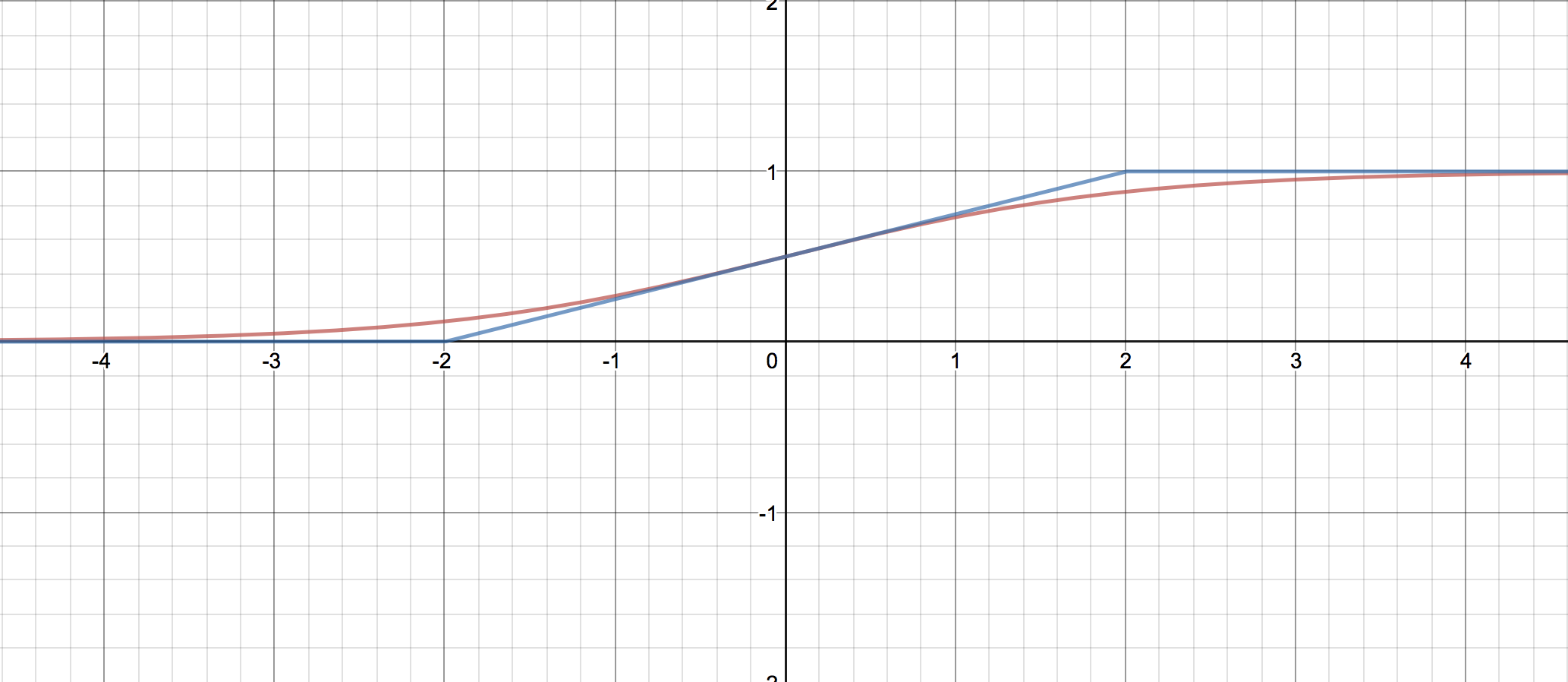
やってみよう。
見てのとおり、0付近での精度は高いものの、±1.5 ~ 3のあたりでの精度の低さが気になる。
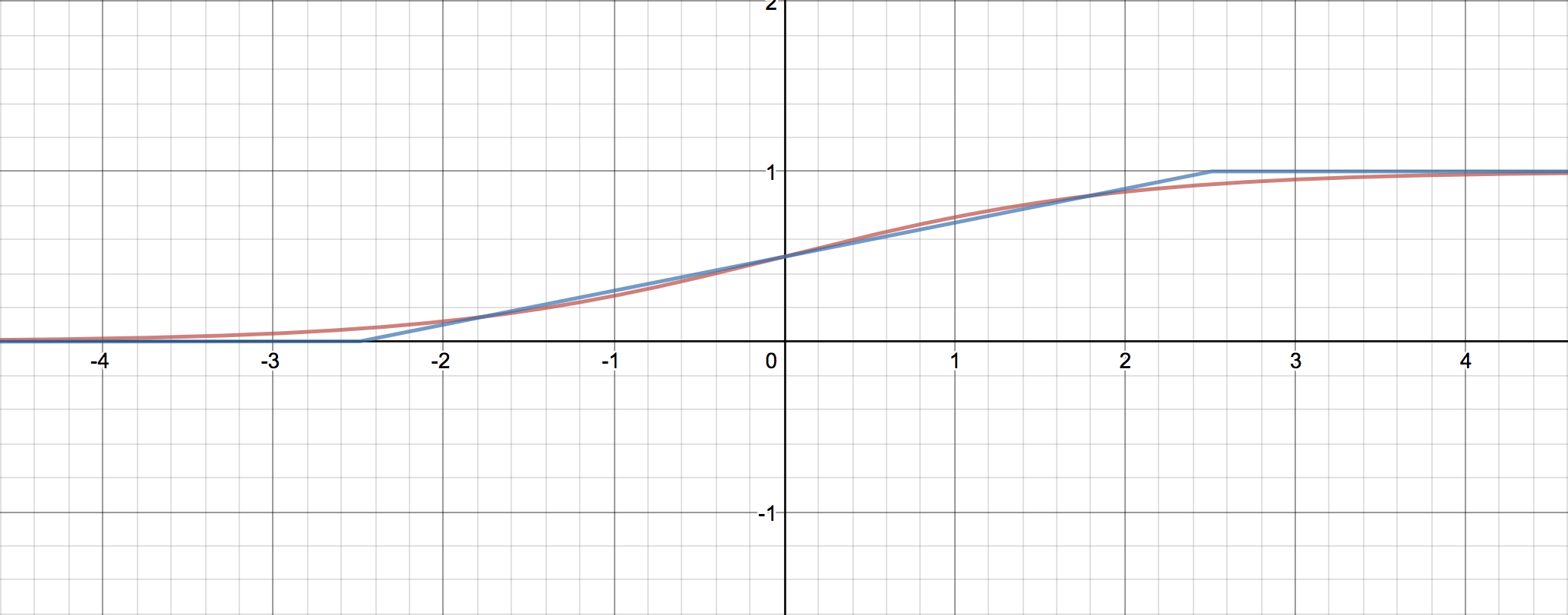
では、傾きを0.25ではなく0.2にしてみるとどうだろう。見てのとおり、比較的広い範囲にわたってシグモイドをそれなりによく近似できているように見える。
ここで終わってもいいのだが
さて、まあ見た目で納得してもらう、というのも手ではあるのだが、それでは0.2という値がマジックナンバーになってしまう。この値にどのような根拠があるのか、調べてみたいものである。
ということで、関数 $g(x)$ を
g(x) = \left\{
\begin{array}{ll}
0 & (x < -a/2) \\
\frac{x}{a} + \frac{1}{2} & (-a/2 \leq x \leq a/2) \\
1 & (a/2 < x)
\end{array}
\right.
と定義して、二乗誤差 $ \int_{-\infty}^\infty \left(f(x) - g(x) \right)^2 dx $ を最小化するような $a$ を求めよう。原点周りでの傾きが $0.2$ に近い値に、つまり、 $a$ が $5$ に近い値になれば成功である。
対称性より、$ \int_{-\infty}^0 \left(f(x) - g(x) \right)^2 dx $ は二乗誤差の半分である。以下これを計算する。
\begin{align}
\int_{-\infty}^0 \left(f(x) - g(x) \right)^2 dx &= \int_{-\infty}^0 \left(f(x)\right)^2 dx - 2\int_{-\infty}^0 f(x)g(x) dx + \int_{-\infty}^0 \left( g(x) \right)^2 dx \\
&= \int_{-\infty}^0 \left(f(x)\right)^2 dx - 2\int_{-a/2}^0 f(x)g(x) dx + \int_{-a/2}^0 \left( g(x) \right)^2 dx \\
&= \int_{-\infty}^0 \left(f(x)\right)^2 dx - 2\int_{-a/2}^0 \frac{e^x}{e^x+1} \left(\frac{x}{a} + \frac{1}{2}\right)dx + \int_{-a/2}^0 \left(\frac{x}{a} + \frac{1}{2}\right)^2 dx
\end{align}
最終行で区分的に定義された関数が登場しなくなったので、これは $a > 0$ において $a$ で微分可能であると推察できる。
第3項 $\int_{-a/2}^0 \left(\frac{x}{a} + \frac{1}{2}\right)^2 dx $ は、 $y = x + \frac{a}{2} $ とすることで
\begin{align}
\int_{-a/2}^0 \left(\frac{x}{a} + \frac{1}{2}\right)^2 dx &= \int_{0}^{a/2} \left(\frac{y}{a} \right)^2 dy = \int_{0}^{a/2} \frac{y^2}{a^2} dy = \frac{1}{a^2} \frac{1}{3}\left(\frac{a}{2}\right)^3 = \frac{a}{24}
\end{align}
と計算できる。ということで、二乗誤差(の半分)を $a$ で微分すると、
\begin{align}
\frac{d}{da}\left( - 2\int_{-a/2}^0 \frac{e^x}{e^x+1} \left(\frac{x}{a} + \frac{1}{2}\right)dx\right) + \frac{1}{24}
\end{align}
これが $0$ となるような $a$ を求めていきたい。
ここで
$$ M(a,x) = 2 \left(\frac{x}{a} + \frac{1}{2}\right) \frac{e^x}{e^x+1} $$
と定義すると、Leibniz integral rule 1
$$ \frac{d}{da} \left(\int_{A(a)}^{B(a)} M(a,x) dx \right)= M\left(a,B(a)\right) \frac{d}{da} B(a) - M\left(a,A(a)\right) \frac{d}{da} A(a) + \int_{A(a)}^{B(a)}\frac{\partial}{\partial a} M(a,x) dx $$
より
$$ \frac{d}{da} \left (\int_{-a/2}^{0} M(a,x) dx \right)= - M\left(a,-\frac{a}{2}\right) \left(-\frac{1}{2}\right) + \int_{-a/2}^{0}\frac{\partial}{\partial a} M(a,x) dx $$
ここで $M\left(a,-\frac{a}{2}\right) = 2 \left(\frac{-a/2}{a} + \frac{1}{2}\right) \frac{e^{-\frac{a}{2}}}{e^{-\frac{a}{2}}+1} = 0$ なので
\begin{align}
\frac{d}{da} \left (\int_{-a/2}^{0} M(a,x) dx \right) &= \int_{-a/2}^{0}\frac{\partial}{\partial a} M(a,x) dx \\
&= \int_{-a/2}^{0} 2 \left(-\frac{x}{a^2} \right) \frac{e^x}{e^x+1} dx
\end{align}
ゆえに、二乗誤差(の半分)を $a$ で微分したものは
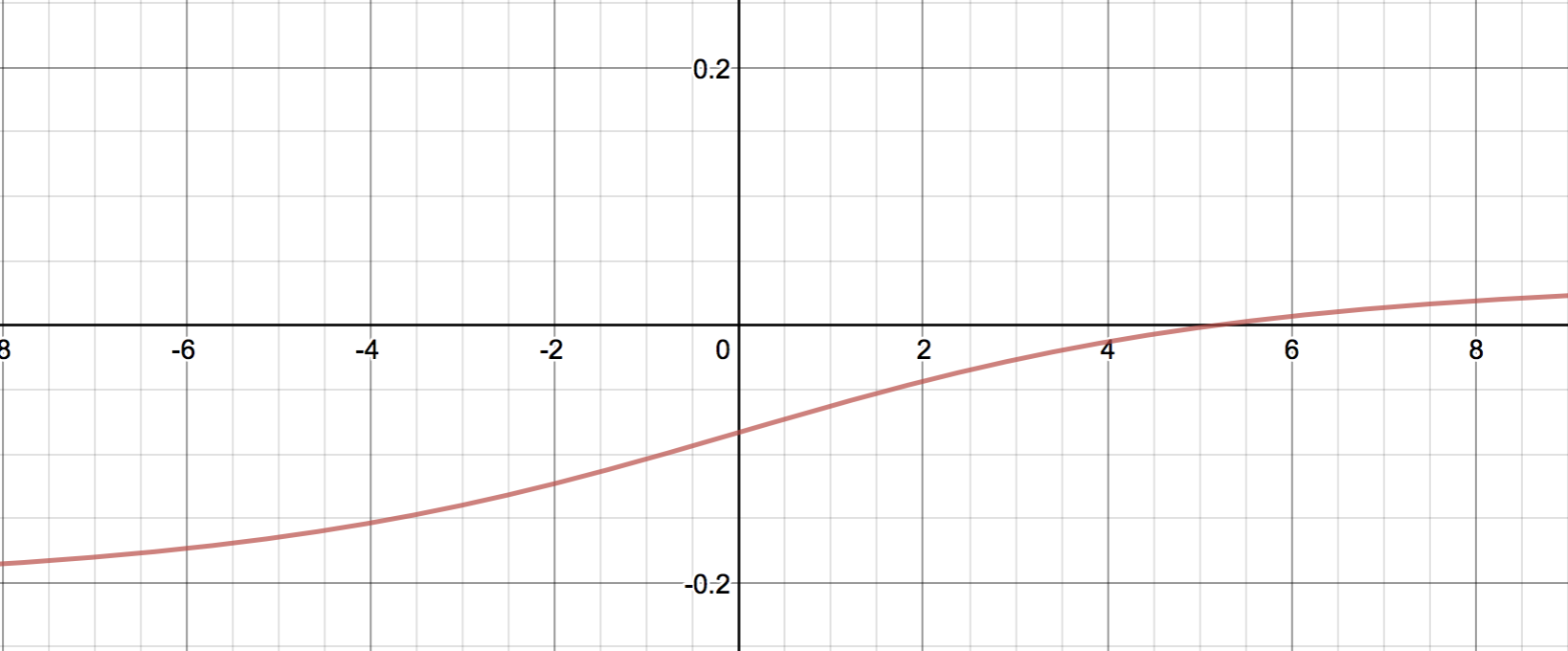
$$ \frac{1}{24} + 2\int_{-a/2}^{0} \frac{x}{a^2} \frac{e^x}{e^x+1} dx $$
と書けることが分かった。これの $a$ についてのグラフを書くと、
たしかに $a=5$ 付近でゼロになっていることが分かる。しかも、一階微分が増加関数であることから、ここが極小であり最小であることも分かる。 2
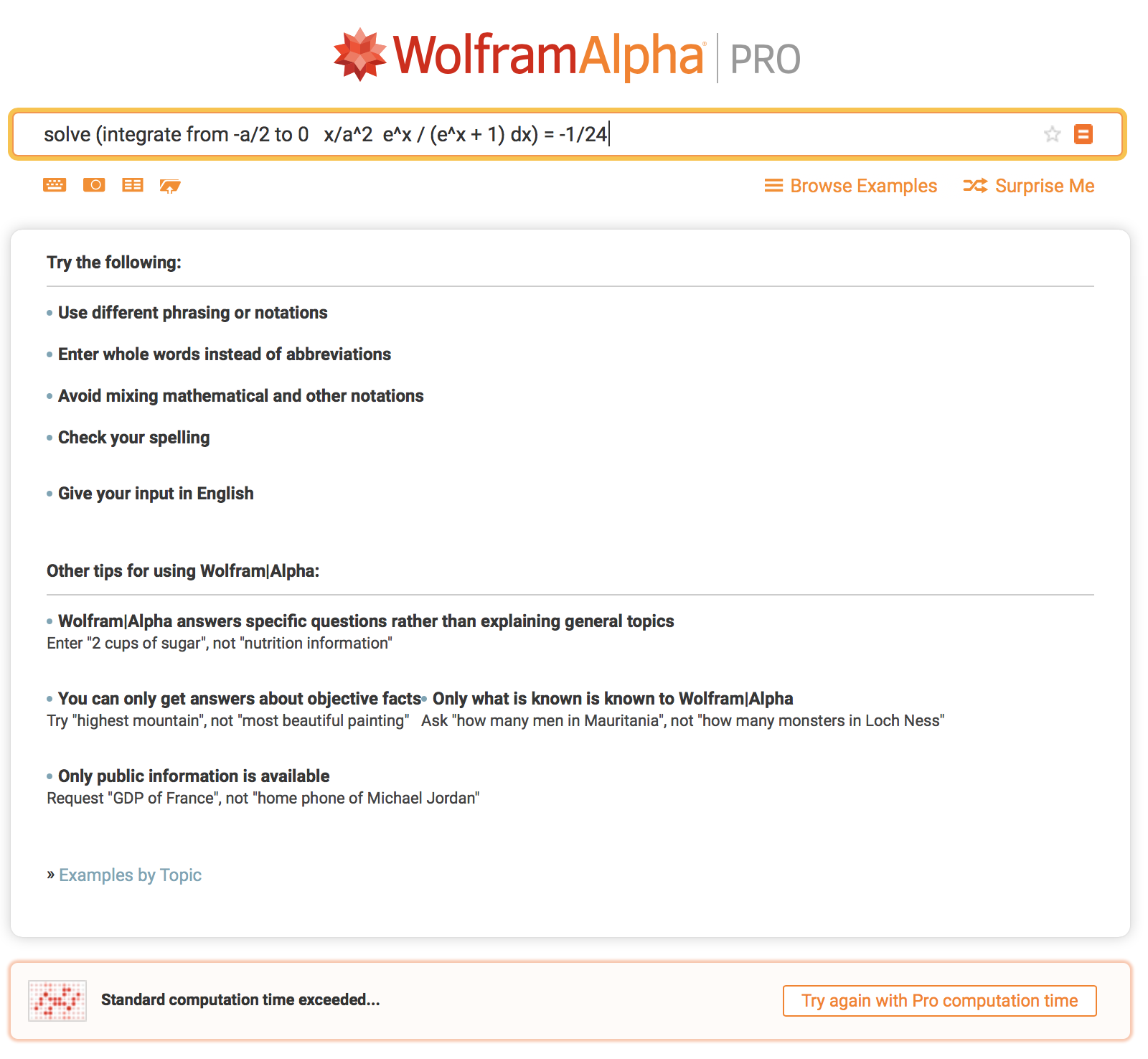
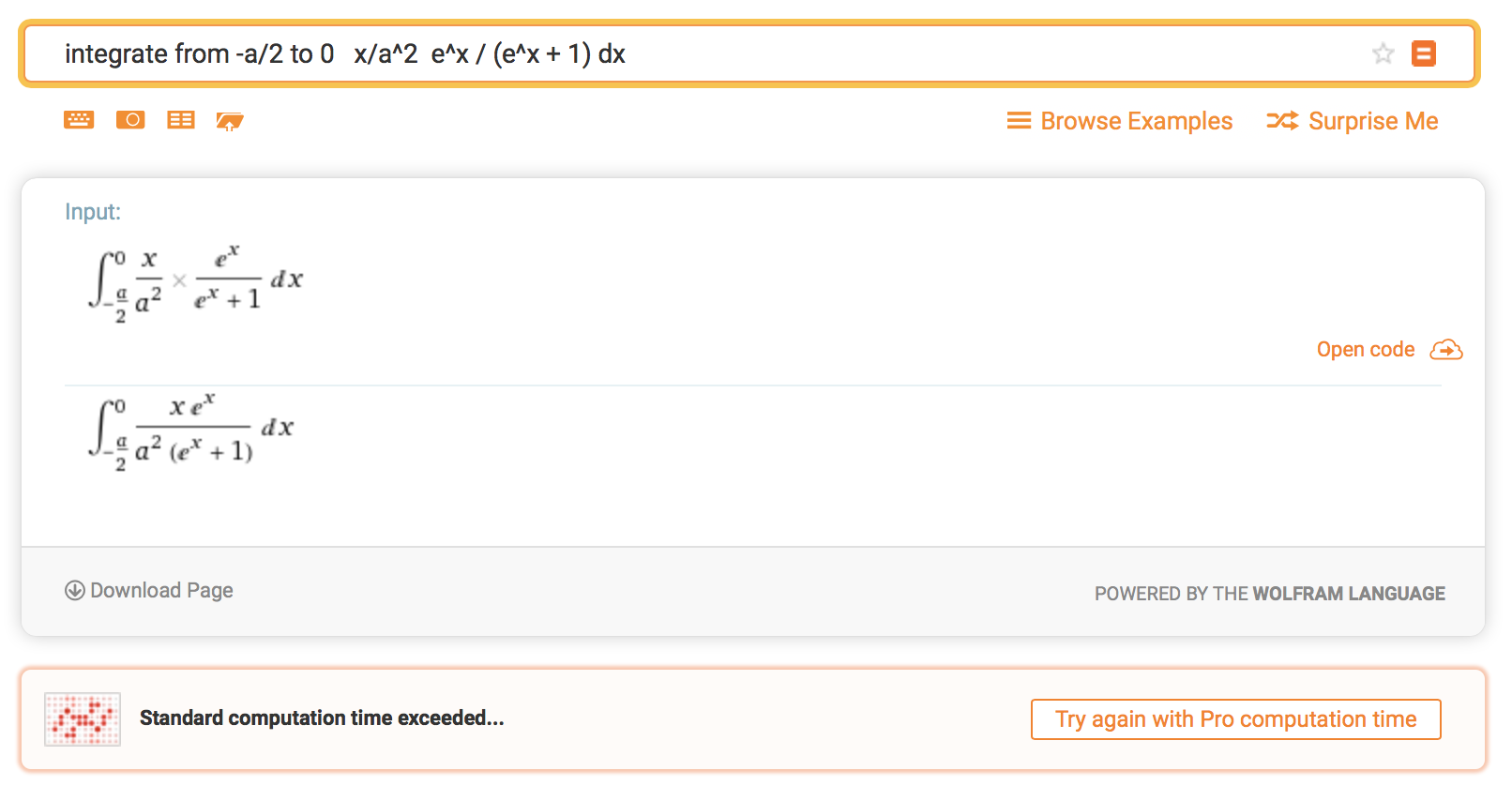
さあ、あとはWolfram Alphaに突っ込んで $a$ を求めるだけ…
うーむ。
じゃあせめて積分だけでも…
(´・ω・`)Wolfram Alphaが読んでくれるように式変形しよう
さて、ということで
$$ 0 = \frac{1}{24} + 2\int_{-a/2}^{0} \frac{x}{a^2} \frac{e^x}{e^x+1} dx $$
を式変形していこう。
$$ \frac{d}{dx} \log(1+e^x) = \frac{\frac{d}{dx} (1+e^x)}{1+e^x} = \frac{e^x}{e^x+1} $$
なので、部分積分により先程の式は
\begin{align}
0 &= \frac{1}{24} + 2 \left. \frac{x}{a^2}  \log(1+e^x)\right|_{x=-a/2}^{x=0} - 2 \int_{-a/2}^{0}  \frac{1}{a^2}  \log(1+e^x) dx \\
&= \frac{1}{24} + \frac{1}{a}  \log(1+e^{-a/2}) - \frac{2}{a^2} \int_{-a/2}^{0}  \log(1+e^x) dx
\end{align}
ここで $u = -e^{x}$ とおくと $du = -e^{x}dx$ なので
\begin{align} \int_{-a/2}^{0} \log(1+e^x) dx = \int_{-e^{-a/2}}^{-1} \log(1-u) \frac{du}{u} \end{align}これは高校数学の範囲では処理できないが、多重対数関数 というものがあって、その中でも $\operatorname{Li}_2(x)$ と呼ばれる関数は負の実数$z$に対して
\operatorname{Li}_2(z) = -\lim_{h \to 0^{-}} \int_h^z \frac{\log(1-u)}{u} duという性質を満たす。
ということで、解くべき式は
0 = \frac{1}{24} + \frac{1}{a} \log(1+e^{-a/2}) + \frac{2}{a^2} \left( \operatorname{Li}_2(-1)- \operatorname{Li}_2(-e^{-a/2}) \right)ということが分かった。ここまで解きほぐしてやればWolfram Alphaも処理することができ、
$$ a = 5.19936381662864... $$
ということが分かる。よって、$x$ に掛ける定数を
$$ \frac{1}{a} = 0.19233122267801... $$
にすると標準シグモイド関数との二乗誤差が最小になることが分かった。
おまけ
hard_sigmoidは $h_1(x) = 1$ と $h_2(x) = 0$ の間を1つの一次関数で繋ぐことで 標準シグモイド関数を近似したが、2つの二次関数で繋いだらどうなるだろう。つまり、
g(x) = \left\{
\begin{array}{ll}
0 & (x < -a) \\
\frac{(x+a)^2}{2a^2} & (-a \leq x < 0) \\
1 - \frac{(x-a)^2}{2a^2} & (0 \leq x \leq a) \\
1 & (a < x)
\end{array}
\right.
とするのである。
この場合、原点での傾きを標準シグモイド関数に合わせる(これは $a = 4$ )のがほぼ最適解となる。詳細は省略するが、
\frac{17}{60} = \frac{4}{a^3} \left(-\frac{a}{2} \operatorname{Li}_2(-e^a) - \frac{a}{2} \operatorname{Li}_2(-1) + \operatorname{Li}_3(-e^a) - \operatorname{Li}_3(-1)\right)を解いて、 $a = 3.99197948719976...$ を得る。
参考文献
- math - How is Hard Sigmoid defined - Stack Overflow ― ソースコードを探すのに直接的に役立った。
- Leibniz integral rule ― これの日本語記事無いの、マジでよろしくないと思うので誰か書いてほしい
追記
Theanoでの原作者はhard_sigmoidの係数が0.2である真の理由を覚えていないらしい、という話があるそうだ。
@fchollet The original author of `hard_sigmoid` in Theano - written 2013 - can't remember. Was it copied in naively from Theano? Estimated based on some assumption of input distribution? Something else?
— Sam Davis (@samgd) 2018年10月15日
この定理は日本語圏で恐ろしく知名度がないようであり、検索しても日本語訳が全然ヒットしない。 ↩
お気づきかもしれないが、今回の問題設定上 $a > 0$ なので、負であるときの振る舞いは関係ない。というかそもそも $a=0$ のときはゼロ除算である。 ↩