- 投稿日:2019-03-10T23:51:00+09:00
Python: Numbaでクラスの高速化
numbaでクラスの高速化.
ただし,クラスの継承はできない模様.また,単純にNumbaに対応させようとしても,意外とコードの手直しが必要がなことは難点であるが,一応投稿.ひとまず,書き方は以下の通り.
spec = [
        ("メンバ変数1", メンバ変数1の型),
        ("メンバ変数2", メンバ変数2の型),
        ....
        ("メンバ変数n", メンバ変数nの型)
    ]

@jitclass(spec)
class ...():
...
from numba import jit, f8, b1, i8, void from numba import jitclass import numpy as np import random spec = [ ("width", i8), ("array", f8[:,:]) ] @jitclass(spec) class test(): def __init__(self, w): self.width = w array = np.array([random.random() for i in range(self.width)]) def start(self): cnt = 0 for a in self.array: cnt += a print(cnt) if __name__ == "__main__": cls = test(10000000) cls.start()
- 投稿日:2019-03-10T23:35:52+09:00
[Python]とにかくわかりやすく!Djangoでアプリ開発!ーその8(最終)ー
前回の記事
[Python]とにかくわかりやすく!Djangoでアプリ開発!ーその7ー
本記事の目的
python初心者の方が、本記事を見たあとに、一人でアプリ開発できることを目的にしております。
※インストールや開発環境については記載しません環境
macOSX Sierra
python3.7
django 2.1.5前回まで
だいぶ長くなってきたので、どのようなことをやってきたか詳細を割愛しますが、たくさんのことをしてきました。
フロントの話やDBの話はまだまだありますが、最低限の機能がついたものとして、公開をしてみたいと思います。
※今回herokuを使いますので事前にherokuのアカウント発行まではしておいてください。絶対に必要なものをインストール
ここら辺はpipで用意します。
$ pip install dj-database-url gunicorn whitenoiserequirements.txtの用意
requirements.txtを用意して、書き込みを行います。
$ pip freeze > requirements.txt中身はこんな感じです。
requirements.txtdj-database-url==0.5.0 Django==2.1.5 django-contrib-comments==1.8.0 gunicorn==19.9.0 psycopg2==2.7.5 whitenoise==4.0そのほか必要なファイルの用意
Procfileとruntime.txtとlocal_setting.pyを用意しておきます。
web: gunicorn myapp.wsgiruntime.txtpython-3.6.6local_setting.pyimport os BASE_DIR = os.path.dirname(os.path.dirname(__file__)) DATABASES = { 'default': { 'ENGINE': 'django.db.backends.sqlite3', 'NAME': os.path.join(BASE_DIR, 'db.sqlite3'), } } DEBUG = True最終的なtreeはこんな感じ
myapp
├── Procfile #ここ
├── db.sqlite3
├── app1
│   ├── __init__.py
│   ├── admin.py
│   ├── apps.py
│   ├── forms.py
│   ├── migrations
│   │   ├── 000x_auto_20190308_2248.py
│   │   └── __init__.py
│   ├── model.txt
│   ├── models.py
│   ├── static
│   │   └── kenko
│   │       └── css
│   │           └── style.css
│   ├── templates
│   │   └── kenko
│   │       ├── create.html
│   │       ├── delete.html
│   │       ├── edit.html
│   │       ├── find.html
│   │       └── index.html
│   ├── tests.py
│   ├── urls.py
│   └── views.py
├── manage.py
├── myapp
│   ├── __init__.py
│   ├── local_settings.py #ここ
│   ├── settings.py
│   ├── urls.py
│   └── wsgi.py
├── requirements.txt #ここ
└── runtime.txt #ここ
settings.pyの修正
settings.pyの最後に以下を追加
settings.pyimport dj_database_url DATABASES['default'] = dj_database_url.config() SECURE_PROXY_SSL_HEADER = ('HTTP_X_FORWARDED_PROTO','https') ALLOWED_HOSTS = ['*'] STATIC_ROOT = 'staticfiles' DEBUG = True try: from .local_settings import * except ImportError: pass STATIC_DIRS = ( os.path.join(BASE_DIR, "static"), )herokuに送る
一応
$ git initログインしてアプリを作ります。
$ heroku login
$ heroku create アプリ名
remoteで接続します。
$ git remote add heroku https://git.heroku.com/アプリ名.gitあとはこんな感じで
$ git add -A
$ git commit -m "commit"
$ git push heroku master
https://<< herokuに登録したアプリ名>>.herokuapp.com
にアクセスしたらアプリは自分のPC以外からも見れるようになっています。補足
デプロイ後にcssが読み込まれなかったので
最後のwhitenoiseを追加したら解決。当然修正のたびにherokuにpushが必要です。settings.pyMIDDLEWARE = [ 'django.middleware.security.SecurityMiddleware', 'django.contrib.sessions.middleware.SessionMiddleware', 'django.middleware.common.CommonMiddleware', 'django.middleware.csrf.CsrfViewMiddleware', 'django.contrib.auth.middleware.AuthenticationMiddleware', 'django.contrib.messages.middleware.MessageMiddleware', 'django.middleware.clickjacking.XFrameOptionsMiddleware', 'whitenoise.middleware.WhiteNoiseMiddleware', ]参照
最後に
約1ヶ月程度をかけてその8まで投稿しました。再度勉強し直したところもありました。
誤字脱字の修正はこれから行います。
本当はバリデーションのこととかDBのこととかまだまだまだまだ内容はありますが、一旦ここで終わりにして、また余裕ができたときに追加をしていきます。
ここまで全部みられたかたがどこまでいらっしゃるかわかりませんが、ありがとうございます。
- 投稿日:2019-03-10T23:01:31+09:00
Python環境構築:Anaconda, Spyder, Visual Studio Code, OpenCV, ffmpeg, Cantera
WindowsでPythonを使い始める
パソコンを新規購入してPythonの環境構築を一からやり直しました.
せっかくなので備忘録として行ったことをまとめておきます.
特にこだわりが無ければ,Anacondaを使いPythonの環境を管理することをお勧めします.
Anacondaをインストールすれば,基本的に環境構築は終了です.
あとはAnaconda promptを使って必要なライブラリを適宜ダウンロード or アップデートするだけです.
以下Anacondaダウンロード先のリンクです.(リンク:Anaconda)
リンクに飛ぶと,上にOSの選択があるのでWindowsを選択してください.
次に2系か3系のPythonの選択がありますが,特にこだわりが無ければ3系を使うことをお勧めします.
(2系と3系ではいくつか書き方を変えないとエラーになるものがあります(e.g. print関数,input関数))エディタとしてSpyderとJupyterがAnaconda navigatorと一緒にインストールされていると思います.
エディタは好みがわかれると思いますが,Visual Studio Codeは試してみる価値はあると思います.
インストール時に選択するポップアップが現れると思いますので,使ってみたければVisual Studio Codeも一緒にインストールしてみてください.
コーディング作業やデバッグ作業は他のエディターよりもはかどる気がします.
OpenCVを使えるようにする
いろいろな方法が記事で取り上げられていますが,ここでは最も簡単な方法を記しておきます.
anaconda promptを開き,以下のコマンドを入力してやるだけです.
conda install -c conda-forge opencvsite-packageのフォルダを確認すればopencvがインストールされていることが確認できると思います.
ffmpegを使えるようにする
動画処理をする際にffmpegを使用することがあると思います.(リンク:FFmpeg)
Pythonからffmpegを使用できるようにするためには,環境変数のシステム環境変数のPathに
「ffmpeg.exe」が存在するフォルダーのパスを追加する必要があります.
コントロールパネル => システム => システム詳細設定から
環境変数を確認するウィンドウを開くことができるので,そこでPathを追加すれば使えるようになります.
Canteraを使えるようにする
燃焼を科学するにあたって,化学反応を解析することがあると思います.
反応速度解析ツールとしてChemkinやCanteraがよく知られていますが,
CanteraはオープンソフトでPythonで実装することができます.(リンク:Cantera python tutorial)
以下のコマンドをAnaconda promptで入力してCanteraライブラリをダウンロードしてみましょう.
conda install -c cantera canteraChemkinのようにGUI化されていないため,使いなれるまでに時間を要しますが無料です.
断熱火炎温度,層流燃焼速度などは簡単に求めることができます.
- 投稿日:2019-03-10T22:27:01+09:00
【fast.ai】 text API解説
概要
本記事はfast.aiのwikiのTextページの要約となります。
筆者の理解した範囲内で記載します。Text モデル、データ、トレーニング
fast.aiライブラリのText モジュールは、DatasetをNLP (Natural Language Processing)目的へ最適化するための関数を多数備えています。具体的には:
- text.transform にてデータの前処理実施し、テキストをidへと変換する
- text.data にて TextDataBunch を用いてNLPに必要なDatasetのクラスを規定する
- text.learner にて素早くlanguage model や RNN classifierを作成できる
上のリンクを辿って各モジュールのAPIを参考にしてみて下さい。
早速やってみる: ULMFiTIでimdbの感情modelを鍛える
早速fast.ai textモジュールを使ってみましょう。以下の例では名の知れたimdbデータを用いて、感情分類モデルを4ステップで鍛えていきます。
1) Imdbデータを読み込み俯瞰する
2) データをモデルに最適化する
3) language modelをfine-tuneする
4) 分類モデルを作成する1) Imdbデータを読み込み俯瞰する
text に必要なパッケージを読み込みましょう。
from fastai.text import *画像認識とは異なり、テキストは直接モデルに読み込むことができません。従って、最初にデータを前処理してテキストをトークンへと変換して(tokenization)それを数字へと変換する(numericalization)必要があります。これらの数字 embedding layer へと引き渡されることで浮動小数点の配列へと変換されます。
これらトークンを浮動小数点へと変換するWord Embeddingsはweb上で掲載されています。これらのWord Embeddingsはwikipediaなどの膨大なサイズのcorpusで鍛えられたものです。ULMFiTの手法を用いて、fast.aiライブラリはpre-trained Language Modelsを用いて、fine-tuneすることに焦点を絞っています。Word embeddingsとは、具体的に300から400の小数点を異なる単語を表すために鍛えられたもので、pre-trained language model はこれらの特性を備えているだけではなく、文や文章を表現する性質も備わっております。
注記: ライブラリは以下の3ステップで構成されています。
- データを最小限のコードで前処理を済ませる
- pre-trained された language model をベースに、データセットを用いてfine-tuneする
- 分類器などのモデルをlanguage modelの上に載せる。
1000レビューに抽出されたIMDBデータセットを用いる(陽性または陰性)
path = untar_data(URLs.IMDB_SAMPLE)
path
PosixPath('/home/ubuntu/.fastai/data/imdb_sample')
データセットをテキストから作成するには以下の方法がベストです
- ImageNet スタイルにフォルダへ整理されている
- csv ファイルへラベルの欄とテキスト欄へ整理されている
こちらの例ではimdbをtexts.csvファイルから読み込んで以下のようになっております。
df = pd.read_csv(path/'texts.csv')
df.head()
label text is_valid 0 negative Un-bleeping-believable! Meg Ryan doesn't even ... 1 positive This is a extremely well-made film. The acting... 2 negative Every once in a long while a movie will come a... 3 positive Name just says it all. I watched this movie wi... 4 negative This movie succeeds at being one of the most u... 2) データをモデルに最適化する
DataBunchを準備するためには、複数のfactory methodsがデータの構成に応じて存在します。詳細はtext.data。こちらでは
from_csvメソッドを用いてTextLMDataBunch(Language Modelのためのデータ処理)とTextClasDataBunch(Text Classifierのためのデータ処理)クラスを用います。# Language model データ処理 data_lm = TextLMDataBunch.from_csv(path, 'texts.csv') # Classifier model データ処理 data_clas = TextClasDataBunch.from_csv(path, 'texts.csv', vocab=data_lm.train_ds.vocab, bs=32)これで必要なデータの前処理がなされます。分類器には、vocabulary(wordからidを引き渡す役目)を引き渡すことによって、data_clasがdata_lmと同じdictionaryを用いる点は注意して下さい。
この処理は時間がかかるため、結果を保存するために以下のコードを実行しましょう。
data_lm.save('data_lm_export.pkl')
data_clas.save('data_clas_export.pkl')
これで全ての結果を保存するための
tmpdirectoryが作成されます。ロードするためには以下のコードを実行しましょう。data_lm = load_data(path, fname='data_lm_export.pkl') data_clas = load_data(path, fname='data_clas_export.pkl', bs=16)注記:
DataBunchのパラメータを設定できます。(batch size,bptt,...)3) language modelをfine-tuneする
data_lmを用いてlanguage modelをfine-tuneしましょう。fast.ai は、AWD-LSTM architectureの英語モデルを用意してるので、それとpretrained weightsをダウンロードし、fine-tuneするためのlearnerオブジェクトを作成しましょうlearn = language_model_learner(data_lm, AWD_LSTM, drop_mult=0.5) learn.fit_one_cycle(1, 1e-2)Total time:00:13
epoch train_loss valid_loss accuracy 1 4.514897 3.974741 0.282455 画像認識モデルと同様に、モデルを
unfreezeすることでさらにfine-tuneすることができます。learn.unfreeze() learn.fit_one_cycle(1, 1e-3)Total time: 00:17
epoch train_loss valid_loss accuracy 1 4.159299 3.886238 0.289092 モデルを評価するために、以下の
Learner.predictを実行することで、単語とその数を指定し予測させることができます。learn.predict("This is a review about", n_words=10)'This is a review about dog - twist credited , and that , along with'
あまり意味は通じませんが(小さいvocabularyのため)ここでは基本的な文法をmodelが習得していることは驚愕すべきことです。(pretrained modelが可能にしたもの)
最後にencoderを保存して分類モデルに用いるようにできるようにしましょう。
learn.save_encoder('ft_enc')4) 分類モデルを作成する
ここでは、先述して作成した
data_clasオブジェクトを用いて、分類器をencoderを用いて新たに作成します。learnerオブジェクト自体はたった一行のコードで作成できます。learn = text_classifier_learner(data_clas, AWD_LSTM, drop_mult=0.5) learn.load_encoder('ft_enc')data_clas.show_batch()
text target xxbos xxmaj raising xxmaj victor xxmaj vargas : a xxmaj review \n \n xxmaj you know , xxmaj raising xxmaj victor xxmaj vargas is like sticking your hands into a big , xxunk bowl of xxunk . xxmaj it 's warm and gooey , but you 're not sure if it feels right . xxmaj try as i might , no matter how warm and gooey xxmaj raising xxmaj negative xxbos xxmaj now that xxmaj che(2008 ) has finished its relatively short xxmaj australian cinema run ( extremely limited xxunk screen in xxmaj xxunk , after xxunk ) , i can xxunk join both xxunk of " xxmaj at xxmaj the xxmaj movies " in taking xxmaj steven xxmaj soderbergh to task . \n \n xxmaj it 's usually satisfying to watch a film director change his style / negative xxbos i really wanted to love this show . i truly , honestly did . \n \n xxmaj for the first time , gay viewers get their own version of the " xxmaj the xxmaj xxunk " . xxmaj with the help of his obligatory " hag " xxmaj xxunk , xxmaj james , a good looking , well - to - do thirty - something has the chance negative xxbos xxmaj to review this movie , i without any doubt would have to quote that memorable scene in xxmaj tarantino 's " xxmaj pulp xxmaj fiction " ( xxunk ) when xxmaj jules and xxmaj vincent are talking about xxmaj mia xxmaj wallace and what she does for a living . xxmaj jules tells xxmaj vincent that the " xxmaj only thing she did worthwhile was pilot " . negative xxbos xxmaj how viewers react to this new " adaption " of xxmaj shirley xxmaj jackson 's book , which was promoted as xxup not being a remake of the original 1963 movie ( true enough ) , will be based , i suspect , on the following : those who were big fans of either the book or original movie are not going to think much of this one negative learn.fit_one_cycle(1, 1e-2)Total time: 00:33
epoch train_loss valid_loss accuracy 1 0.650518 0.599687 0.691542 再度modelをunfreezeしてfine-tuneしましょう。
learn.freeze_to(-2)
learn.fit_one_cycle(1, slice(5e-3/2., 5e-3))
Total time: 00:38
epoch train_loss valid_loss accuracy 1 0.628320 0.563579 0.716418 learn.unfreeze() learn.fit_one_cycle(1, slice(2e-3/100, 2e-3))Total time: 00:56
epoch train_loss valid_loss accuracy 1 0.533411 0.539693 0.721393 そして、
Learner.predictを用いてテキストを予測してみましょう。learn.predict("This was a great movie!")(Category positive, tensor(1), tensor([0.0118, 0.9882]))
- 投稿日:2019-03-10T22:00:03+09:00
【Ubuntu】WebRTCで色々画像処理して遊ぶ【Flask】
目的
WebRTCを使って、Web上からPCやスマホのカメラから映像取得して、それをWebサーバに送信。サーバ側で画像処理して、ユーザ側には画像を返すなり何かしらパラメータ返すなりする。
例えばスマホで撮った映像から物体検出等をリアルタイムですることができる。開発環境
- OS
- Ubuntu16.04.5(AWSのEC2使用)
- 言語
- Python3.5.2
- Flask
- OpenCV
- HTML5
- JavaScript
- WebRTC
- JQuery
WebRTCを使用する際はSSL通信化しておく必要があります。flaskのSSL通信化については私が以前書いたものを参考にしてください。
【Ubuntu16.04.5】PythonのFlaskをHTTPS化処理の流れ
WebRTCによるカメラ映像取得
いつのバージョンからか、WebRTCを使用する際はasyncを使用しなければならないようです。
調べても大体async使ってないソースばっかりで、エラーに悩まされてました。公式のサンプルソースコードをしっかり読みましょう[1]。映像取得だけなら以下の部分だけで十分です(多分)。(#myvideoはvideoタグ、#startはボタンタグ)
ただし停止ボタンが無いので延々とブラウザにカメラ映像が表示されます。停止するならリロードなり何なりしてください。$(function(){ const constraints = window.constraints = { audio: false, video: { facingMode: "environment" } }; async function init() { try { const stream = await navigator.mediaDevices.getUserMedia(constraints); const video = document.querySelector('#myvideo'); const videoTracks = stream.getVideoTracks(); window.stream = stream; video.srcObject = stream; e.target.disabled = true; } catch{ $('#errorMsg').text('カメラの使用を許可してください'); } } $('#start').click(init); });
facingModeでは、デフォルトで使用されるカメラを指定しています。"environment"でフロントカメラ、"user"でインカメラを指します。未指定なら後者になります。映像を処理用URLに送信
ぶっちゃけ参考文献[2]丸パクリです(リンク先はWebRTCからtensorflowの物体検出してる)。
流れとしては
- canvasタグに一旦描画する
- canvasタグから画像バイナリデータ取得する
- データをAjaxで処理先に送信する
となります。以下のように実装しました。
    var canvas = $('#videocanvas')[0];

    $('#myvideo').on('loadedmetadata', function(){
        // canvasのサイズ合わせ
        var video = $('#myvideo')[0];
        var width = canvas.width = video.videoWidth;
        var height = canvas.height = video.videoHeight;

        // 描画先の指定
        var ctx = canvas.getContext("2d");

        // 送信データの作成
        var fd = new FormData();
        fd.append('video', null);

        //毎フレーム処理
        setInterval(function(){
            ctx.drawImage(video, 0, 0, width, height);
            canvas.toBlob(function(blob){

                fd.set('video', blob);

                $.ajax({
                    url: "/img",
                    type : "POST",
                    processData: false,
                    contentType: false,
                    data : fd,
                    dataType: "text",
                })
                .done(function(data){
                    console.log(data);
                })
                .fail(function(data){
                    console.log(data);
                });
            }, 'image/jpeg');
        },1000);
    });
.on('loadedmetadata'はvideoタグの読み込みが終わった時に実行する処理ということです。つまりはカメラに正常にアクセスできた場合ということですね。
そこからsetIntervalを使って定期的に送信していきます。処理部
@api.route("/img", methods=["POST"])
def img():
    img = request.files["video"].read()

    # pillow から opencvに変換
    imgPIL = Image.open(io.BytesIO(img))
    imgCV = np.asarray(imgPIL)

    imgCV = cv2.bitwise_not(imgCV)

    # 好きな処理を入れる

    return "success"
まあぶっちゃけここはお好きにしてください。私はOpenCV使うので変換挟んでます。
処理後の画像を描画したい
Flaskにはもともとimgタグでストリーミングできる仕組みが存在します[3]。
なのでそれを使えば実現できます。app.py(一部)@api.route('/feed') def feed(): return Response(gen(), mimetype='multipart/x-mixed-replace; boundary=frame') def gen(): while True: with open('./templates/dst/test.jpg', 'rb') as f: img = f.read() yield (b'--frame\r\n' b'Content-Type: image/jpeg\r\n\r\n' + img + b'\r\n')index.html(一部)<img id="preview" src="{{ url_for('feed') }}"><br>こうして、あとは処理した画像を
test.jpgに保存すれば解決。まとめ
(ぶっちゃけWebでやる必要ある?)
メリットとしては同じ精度や処理速度をスペックの異なるスマホ等で実現できる・・・ということくらいですかね。ただAWSのデフォルトサーバ程度では大した利点は無いです。
特徴点マッチング使った処理で、大体5アクセスの時点でCPU100%になってレスポンス遅くなりましたね。よっぽどのつよつよサーバじゃないとネイティブアプリで実現する方がいいかと思います。ちなみにそもそもレスポンスは遅いです。大体1秒くらい。
参考文献
[1]getUserMedia(Sample Code)
[2]Computer Vision on the Web with WebRTC and TensorFlow - webrtcHacks
[3]FlaskとOpenCVを使ってWEBカメラで撮影した画像をストリーミングする - Qiita
- 投稿日:2019-03-10T21:59:36+09:00
SUUMOのお買い得中古不動産TOP30 by GCN
ゴール
GCNを使ってSUUMOからお買い得物件TOP30を見つけちゃいます
背景
ReNomというサイトでこんなGCNを使った不動産関連のチュートリアルがあり、簡単にできそうだったので勉強がてらやってみました。全ソース公開します。
対象読者
python始めたばかりの方
東京都内の中古不動産購入予定者方法
肝心なGCN部分はチュートリアルをまんまパクって、データはSUUMOの東京中古不動産情報から引っ張ってくるというやり方です。
大まかな流れは以下の通り。
- スクレイピング
- 前処理
- 学習
- 結果確認
- appendix
環境
python3
jupyter labライブラリ
ReNom,ReNomRG,BeautifulSoup等
ポイント
今回は、駅名・路線名のような情報を単純にワンホット化(数値データでないデータを0,1のみで表現する方法)するのではなく、
ターゲットエンコーディングという方法を使用しました。
ワンホットだと駅の数、路線の数に応じて変数の数が増えてしまうので、計算に時間かかります。
ワンホットで試しにやってみたところ、変数が多すぎて自分のMacbook air '11 メモリ4GB (貧弱...)では標準化できずにフリーズしました。
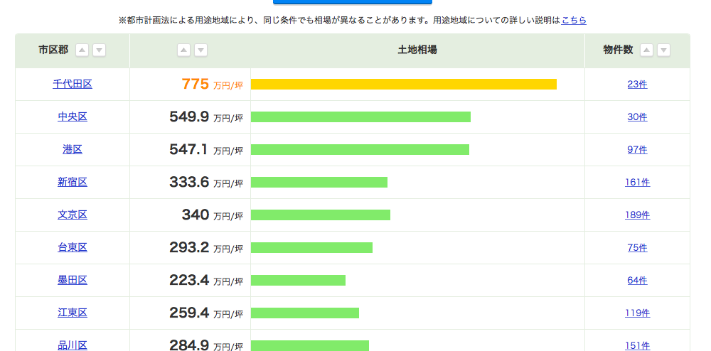
具体的には、suumoさんは駅毎の坪単価と路線毎の坪単価を持っているので、駅名と路線名をこの坪単価で置き換えます。1. スクレイピング
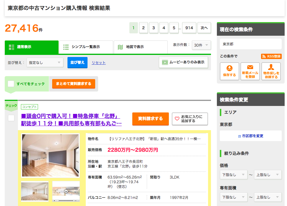
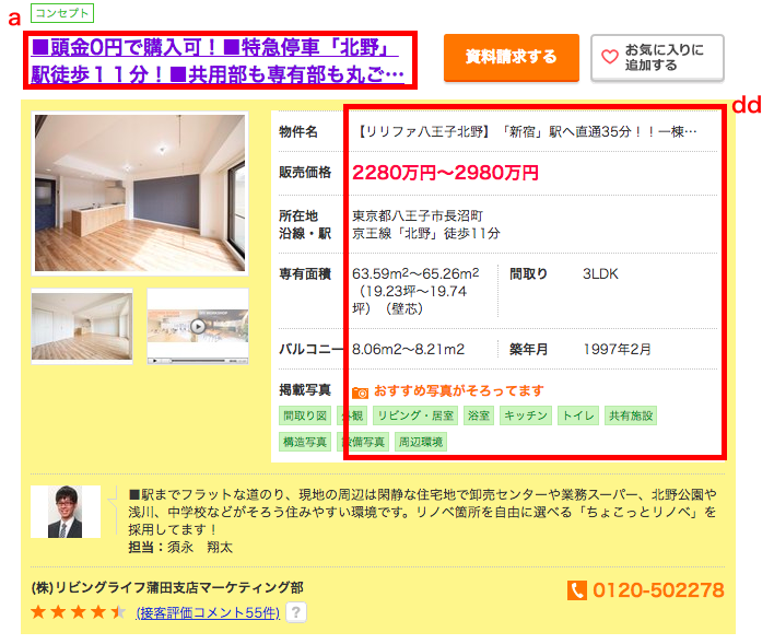
東京都内のSUUMOに掲載されている中古不動産全件を取得します。
まずは上図のページ情報を取得します。
#必要なライブラリをインポート
from bs4 import BeautifulSoup
import requests
import pandas as pd
from pandas import Series, DataFrame
import time
import datetime
import numpy as np
import scipy.stats
from sklearn import preprocessing
from tqdm import tqdm

#東京都の中古マンション一覧
url = 'https://suumo.jp/jj/bukken/ichiran/JJ010FJ001/?ar=030&bs=011&ta=13&jspIdFlg=patternShikugun&kb=1&kt=9999999&mb=0&mt=9999999&ekTjCd=&ekTjNm=&tj=0&cnb=0&cn=9999999'

#データ取得
result = requests.get(url)
c = result.content

#HTMLを元に、オブジェクトを作る
soup = BeautifulSoup(c)
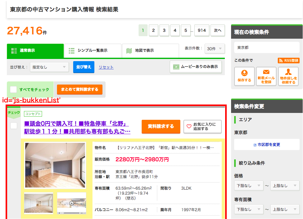
soupにこのページ(1ページ目の)情報が格納されました。
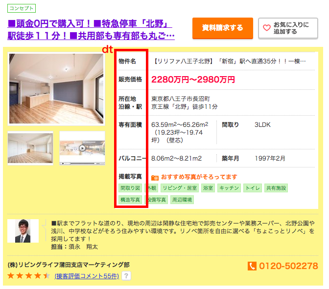
このページからid='js-bukkenList'(このページの不動産情報全件)を取得し、そこから各物件の価格を予想する際の説明変数名を取得します。
#物件リストの部分を切り出し
summary = soup.find("div", id='js-bukkenList') #1ページ分を取得
dt = summary.find("div",class_='ui-media').find_all('dt') #dtを全て取得
cols = [t.text for t in dt]
cols.insert(0, 'url') #後ほど物件情報詳細を確認するためurl列を追加
次にページ数を取得し、2ページ目以降のurlを生成していきます。
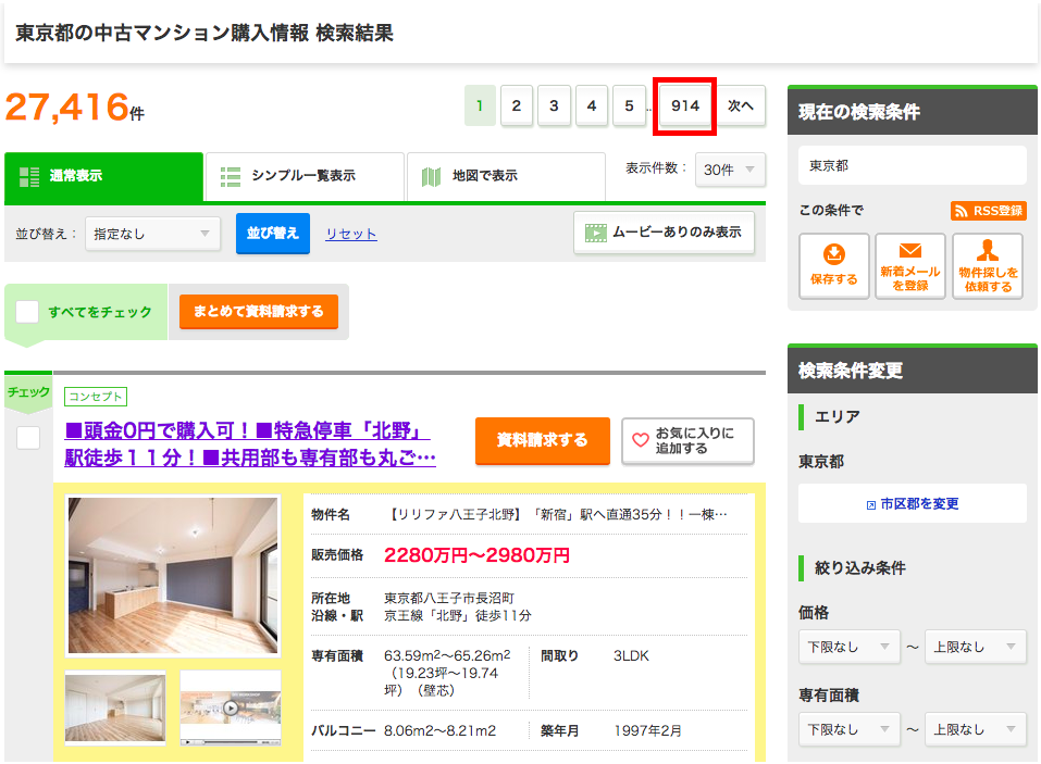
#ページ数を取得
body = soup.find("body")
page = body.find("div",class_='pagination pagination_set-nav')
li = page.find_all('li')
pg_length = int(li[-1].text)

#URLを入れるリスト
urls = []

#1ページ目を格納
urls.append(url)

#2ページ目から最後のページまでを格納
for i in range(pg_length)[:-1]:
    pg = str(i+2) #2ページ目から
    url_page = url + '&pn=' + pg #ページ数に合わせたurl
    urls.append(url_page)
全ページのurlを生成出来ました。
ここから全ページ
の物件情報(aタグとddタグ情報)を取得していきます。
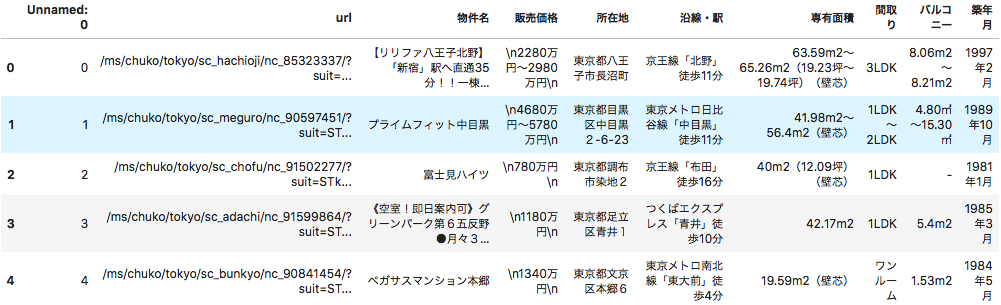
#各ページで以下の動作をループ
bukkens =[]
for url in tqdm(urls):
    #物件リストを切り出し
    result = requests.get(url)
    c = result.content
    soup = BeautifulSoup(c)
    summary = soup.find("div",id='js-bukkenList')

    #マンション名、住所、立地(最寄駅/徒歩~分)、築年数、建物高さが入っているproperty_unitsを全て抜き出し
    property_units = summary.find_all("div",class_='property_unit-content')

    #各property_unitsに対し、以下の動作をループ
    for item in property_units:
        l = []
        #マンションへのリンク取得
        h2 = item.find("h2",class_='property_unit-title')
        href = h2.find("a").get('href')
        l.append(href)
        for youso in item.find_all('dd'):
            l.append(youso.text)
        bukkens.append(l)
    time.sleep(0.5)
東京都内の不動産情報全件を
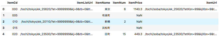
bukkensに格納しました。これを一旦csvに出力します。#列名を設定し、csvに一旦export df = pd.DataFrame(bukkens,columns=cols) df.to_csv('bukken.csv') #csvのimportと中身の確認 df = pd.read_csv('bukken.csv') df[0:5]ここまででスクレイピングは完了です。取得したデータはこんな感じでDataFrameに格納されています。
2.前処理
各列のデータから余分な文字列を除去していきます。
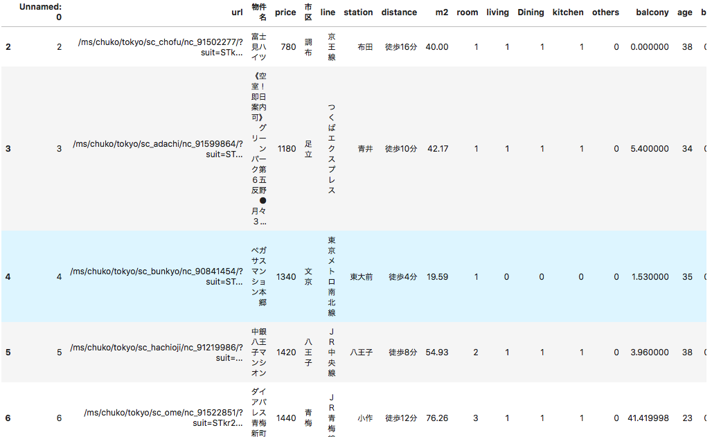
#販売価格に「〜」が含まれている行を削除
df = df[~df['販売価格'].str.contains('~')]
#価格を値のみへ
# _df = df['販売価格'].str.extract('\n([億0-9]+)万円') #seriesじゃないとstr使えない
_df = df['販売価格'].str.extract('(.+)[億]+').astype(float).fillna(0)*10000
_df2 = df['販売価格'].str.extract('[\n|億]([0-9]+)万円').astype(float).fillna(0)
df['price'] = _df + _df2
#price列に欠損があれば、drop
df.dropna(subset=['price'],inplace=True)
df['price'] = df['price'].astype(int)
df = df[df['price'] != 0]

#市区最寄り駅を求める
df['市区'] = df['所在地'].str.extract('都(.+)[市|区]')
df[['line','station','distance']] = df['沿線・駅'].str.extract('(.+)「(.+)」(.+)')
#専有面積
df['m2'] = df['専有面積'].str.extract('([\d\.]+)m2').astype('float')
#間取り
df['room'] = df["間取り"].str.extract('(\d+).+').fillna(1).astype('int')
df['living'] = df["間取り"].str.count('L')
df['Dining'] = df["間取り"].str.count('D')
df['kitchen'] = df["間取り"].str.count('K')
df['others'] = df["間取り"].str.count('S')
#バルコニー
df['balcony'] = df['バルコニー'].str.extract('([\d\.]+)m2').fillna(0).astype('f4')
#築年数
year = datetime.date.today().year
df['age'] = year - df['築年月'].str.extract('(.+)年').astype('int')

#不要列削除
df2 = df.drop(['販売価格','所在地','沿線・駅','専有面積','間取り','バルコニー','築年月'],axis=1)

#バスと徒歩の時間を抽出
df2['bus'] = df2['distance'].str.extract('バス(\d+)分').astype(float)
df2['walk'] = df2['distance'].str.extract('歩(\d+)分').astype(float)
#それぞれ欠損を穴埋め
df2[['bus','walk']] = df2[['bus','walk']].fillna(0)
df2[0:5]
一旦
df2に余分な文字が除去されたデータを格納しました。
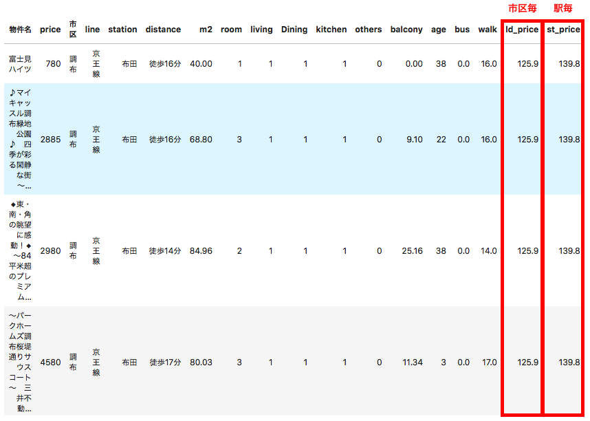
ここであらかじめSUUMOから取得しておいた市区毎の平均坪単価、駅毎の平均坪単価を説明変数に加えます。これがターゲットエンコーディングです! 取得方法についてはappendixを見てください。#区毎の坪単価の読み込み lp = pd.read_csv('land_price.csv') lp['市区'] = lp['itemName'].str.extract('(.+)[市|区|郡]') lp = lp.drop(['Unnamed: 0', 'itemName'],axis=1) lp.columns = ['ld_price','市区'] #駅毎の坪単価の読み込み sp = pd.read_csv('station_price.csv') sp['station'] = sp['itemName'] sp = sp.drop(['Unnamed: 0', 'itemName'],axis=1) sp.columns = ['st_price','station'] #市区毎、駅毎の坪単価平均をマージ df2 = pd.merge(df2, lp, on='市区') df2 = pd.merge(df2, sp, on='station') df2[0:5]マージした結果がこちらです。
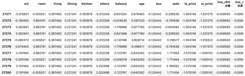
再右列にデータが追加されています。駅毎の平均坪単価が算出されていないケースについては市区毎の平均坪単価を代用します。#駅の平均坪単価が算出されていない場合は市区平均坪単価を代用 df2.loc[df2['st_price'].isnull(), 'st_price'] = df2['ld_price']ワンホット化(路線名のみ)、標準化を行います。
#不要列を削除し、ワンホット化
df3 = pd.get_dummies(df2.drop(['url','物件名','市区','station','distance'],axis=1))
df3.info()

#標準化
temp = df3.iloc[:,2:]
df4 = (temp - temp.mean()) / temp.std(ddof=0)
print(df4.isnull().any(axis=0).sum())
df4[-10:]
前処理が完了しました。
結果がこちらです。路線名がワンホットされており、その他についても標準化されています。
ようやく準備完了!
3.学習
学習用とテスト用にデータを分けます。
後から行番号を使いたいので、indicesをtrain_test_splitの引数に設定します。#学習用(`~train`)とテスト用(`~test`)にデータ分割 from sklearn.model_selection import train_test_split X = df4.values y = df3['price'].values indices = df3['Unnamed: 0'].values X_train, X_test, y_train_org, y_test_org, i_train, i_test = train_test_split(X, y, indices, test_size=0.2) y_train = np.log(y_train_org)#logにすることにより不動産価格の差異が小さくなり、精度が上がる y_test = np.log(y_test_org)ここからはGCNを使ったチュートリアルをそのまま使っています。
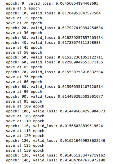
#ハイパーパラメータの設定(参考元チュートリアルのまま)
epoch = 100
batch_size = 16
num_neighbors = 5
channel = 10

#ReNomのGCNNを使用
import renom as rm
from renom.optimizer import Adam
from renom_rg.api.regression.gcnn import GraphCNN
from renom_rg.api.utility.feature_graph import get_corr_graph, get_kernel_graph, get_dbscan_graph
#インデックス行列の取得
index_matrix = get_corr_graph(X_train, num_neighbors)

#GCNNのレイヤーの定義
model = rm.Sequential([
    GraphCNN(feature_graph=index_matrix, channel=channel, neighbors=num_neighbors),
    rm.Relu(),
    rm.Flatten(),
    rm.Dense(1)
])

#最適化関数はAdam
optimizer = Adam()

#学習
train_loss_list = []
valid_loss_list = []

for e in range(epoch):
        N = X_train.shape[0]

        perm = np.random.permutation(N)
        loss = 0
        total_batch = N // batch_size

        for j in range(total_batch):
            index = perm[j * batch_size: (j + 1) * batch_size]
            train_batch_x = X_train[index].reshape(-1, 1, X_train.shape[1], 1)
            train_batch_y = y_train[index]

            # Loss function
            model.set_models(inference=False)
            with model.train():
                batch_loss = rm.mse(model(train_batch_x), train_batch_y.reshape(-1, 1))

            # Back propagation
            grad = batch_loss.grad()

            # Update
            grad.update(optimizer)
            loss += batch_loss.as_ndarray()

        train_loss = loss / (N // batch_size)
        train_loss_list.append(train_loss)

        # validation
        model.set_models(inference=True)
        N = X_test.shape[0]

        valid_predicted = model(X_test.reshape(-1, 1, X_test.shape[1], 1))
        valid_loss = float(rm.mse(valid_predicted, y_test.reshape(-1, 1)))
        valid_loss_list.append(valid_loss)

        if e % 5 == 0 and valid_loss < valid_loss_list[e - 1]:
            model.save("model1.h5")
            print('save at', e, 'epoch')

        if e % 10 == 0:
            print("epoch: {}, valid_loss: {}".format(e, valid_loss))
学習結果はこのようになりました。
4.結果確認
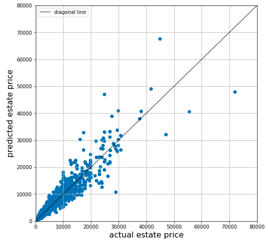
テスト(
test)用のデータ(実際の不動産価格)とGCNNが予測した不動産価格(predict)を比較します。#予測と実際の価格の比較 test = np.exp(y_test) predict = np.exp(valid_predicted) plt.figure(figsize=(8, 8)) plt.plot([0, 80000], [0, 80000], c='k', alpha=0.6, label = 'diagonal line') # diagonal line plt.scatter(test, predict) # plt.scatter(registered_true, registered_pred,label='registered') plt.xlim(0, 80000) plt.ylim(0, 80000) plt.xlabel('actual estate price', fontsize=16) plt.ylabel('predicted estate price', fontsize=16) plt.legend() plt.grid()概ね予測した不動産価格と実際の不動産価格の差異が小さいことがわかります。
モデルは完成したので、全データに対して予測をしてみましょう!
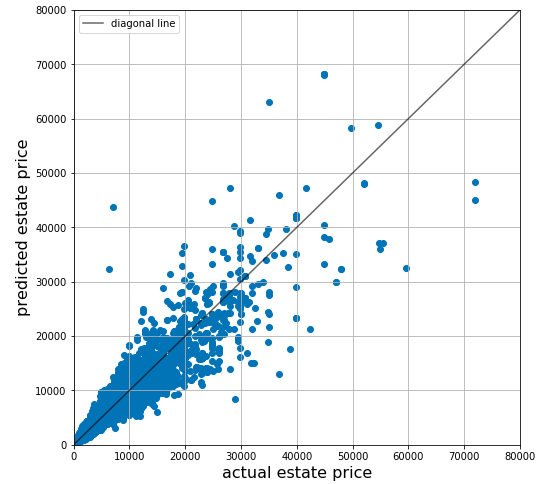
#一度モデルのパラメータをリセット
for layer in model:
    setattr(layer, "params", {})

#学習時に保存したweightを読み込み
model.load("model1.h5")

#全物件に対しGCNNで予測を行う。
log_predict = model(X.reshape(-1, 1, X.shape[1], 1))
GCNNの予測結果を確認しましょう。
#実際の価格と予測の比較
import matplotlib.pyplot as plt
predict = np.exp(log_predict)

plt.figure(figsize=(8, 8))
plt.plot([0, 80000], [0, 80000], c='k', alpha=0.6, label = 'diagonal line') # diagonal line
plt.scatter(y, predict)
plt.xlim(0, 80000)
plt.ylim(0, 80000)
plt.xlabel('actual estate price', fontsize=16)
plt.ylabel('predicted estate price', fontsize=16)
plt.legend()
plt.grid()
全データに対しての予測結果はこちらです。若干ばらつきが出てますね〜。。
ここからお待ちかねのお買い得物件リストアップです!
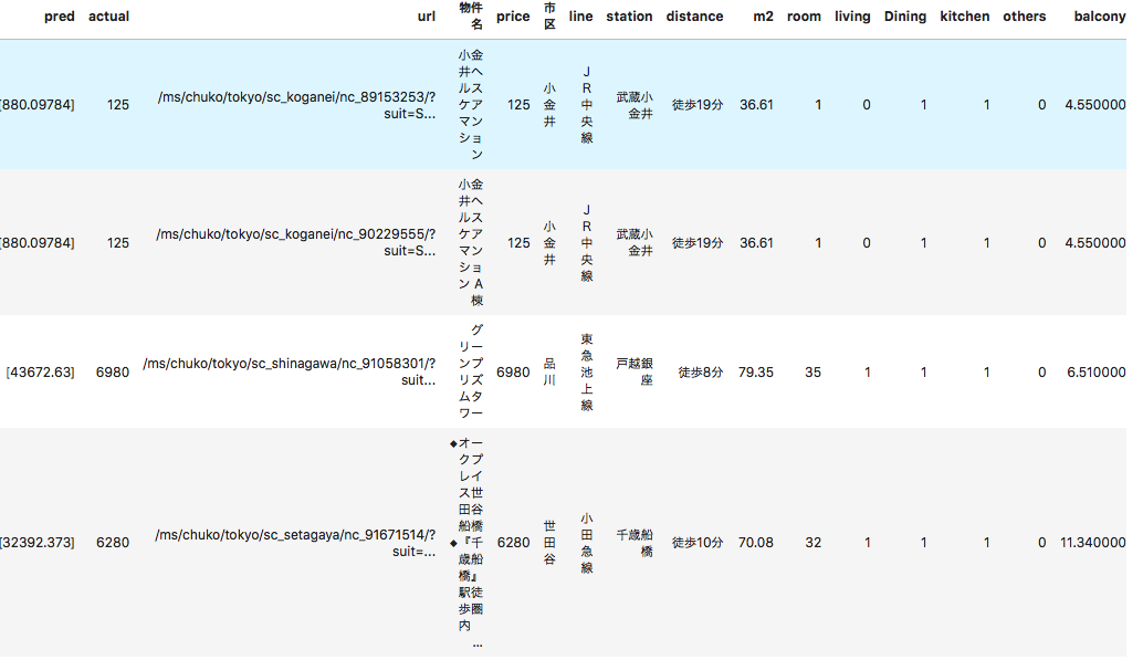
#実際の価格に対して予測がどれだけ乖離しているか(どれだけお得かどうか)の算出
df5 = pd.DataFrame([indices, predict, y]).T
df5.columns=['Unnamed: 0', 'pred', 'actual']
df5['Unnamed: 0'] = df5['Unnamed: 0'].astype(int)
df6 = pd.merge(df5, df2, on='Unnamed: 0')
df6['diff'] = df6['pred'] - df6['actual']
df6['proportion'] = df6['diff'] / df6['actual']

#予測が実際の価格から50%以上乖離している物件
df7 = df6[abs(df6['proportion']) > 0.5].sort_values('proportion', ascending=False)
#お買い得物件TOP10
df7[0:9]
上位はこれです!
predが不動産価格の予測結果,actualが実際の価格を表しています。
1番お買い得な物件は実際の価格の約6倍との結果となっています。確かに125万円は安いのでは?
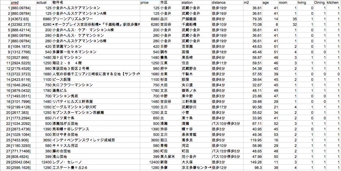
TOP30の結果をみてみましょう。
No.3戸越銀座とNo.4千歳船橋は上の図にも出てますが、35LDK,32LDKあることになってますね〜それは予測が4億になる。
こういう記載誤りにも気づけますね
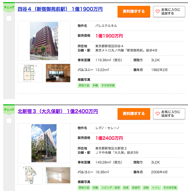
個人的に気になったNo.29の新宿の物件レグノ・セレーノを見てみましょう
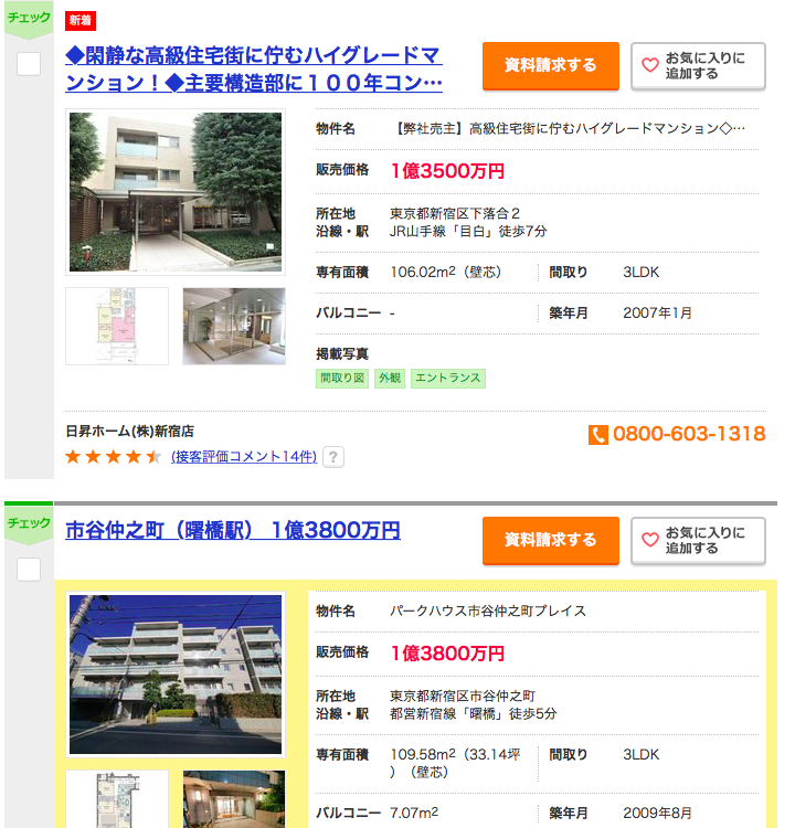
似た条件(新宿区、100平米以上、3K以上、駅徒歩7分以内)で検索してみました。
こちら
この広さ、築年数、駅徒歩分数でこの値段は安い気がしませんか?決して買えないですが、、、
5.まとめ
ReNomを使い、こんなに簡単にお得な物件を見つけることができました!
お金のある方はNo.29の新宿の物件レグノ・セレーノを買っちゃうのはありではないでしょうか。笑
一切責任は追えませんが、、まだ階数や複数の最寄駅情報のようなそのほかの定量的情報は取れていないので、精度向上の余地はまだまだあります。内装の雰囲気、治安のような定性的情報も追加できれば、まさに不動産テックといえるレベルになりますね。
Appendix
市区毎の平均坪単価と駅毎の坪単価平均を取得します。
市区毎の坪単価平均
こちらもSUUMOから情報を取得します。
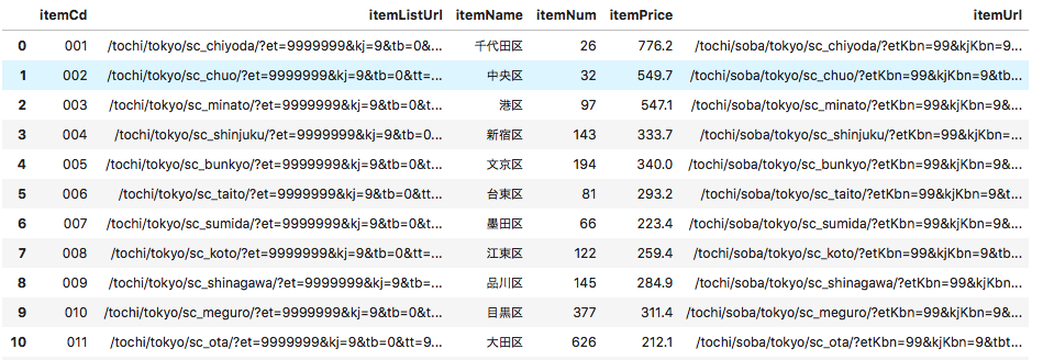
#必要なライブラリをインポート
from bs4 import BeautifulSoup
import requests
import pandas as pd
from pandas import Series, DataFrame

#東京都市区毎の坪単価情報掲載ページ
url = 'https://suumo.jp/tochi/soba/tokyo/area/'

#データ取得
result = requests.get(url)
c = result.content

#HTMLを元に、オブジェクトを作る
soup = BeautifulSoup(c)

#市区毎のデータ平均坪単価情報はid='js-graphData'から取得
#scriptタグ内にjson形式でデータが存在する
body = soup.find("script", id='js-graphData')

#取得したbodyに含まれる余分な'\r\n'を削除
body_text = body.text.replace('\r\n', '')
json形式のデータを読み込む
import json
body_json = json.loads(body_text)

#dataframeにつっこむ
landPrice = pd.DataFrame(body_json)
#itemNum(平均坪単価の値)がnullなところには0で補間
landPrice['itemNum'][landPrice['itemNum']=='']=0
#itemNumが0より大きい市区のみのデータを利用
landPrice = landPrice[landPrice['itemNum'].astype(int)>0]

#csvに出力
landPrice[['itemName','itemPrice']].to_csv('land_price.csv')
landPriceの中身はこんな感じ。
駅毎の坪単価平均
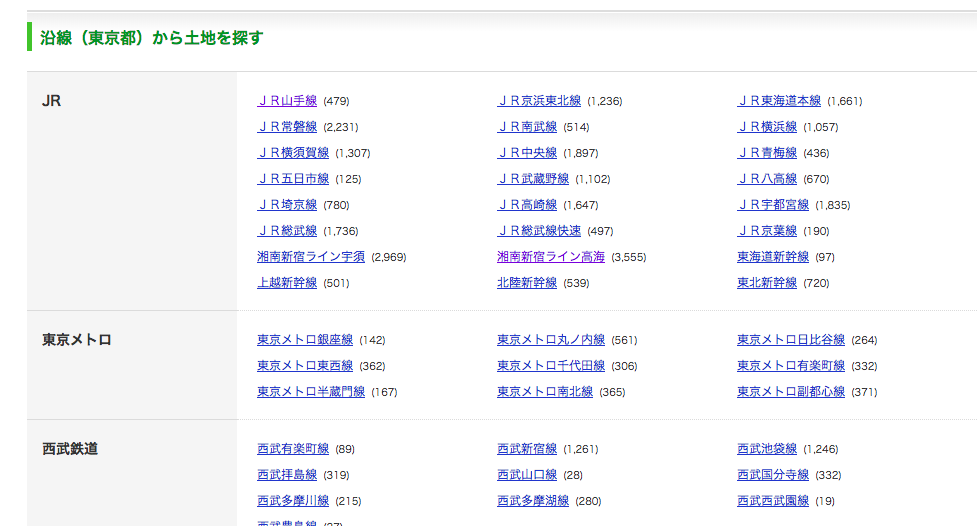
こちらもSUUMOから情報を取得します。
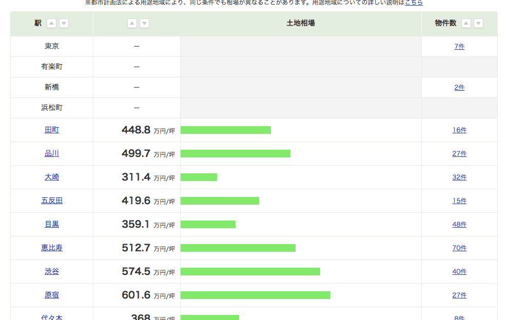
このページのJR山手線をクリックすると、
のページが開き、市区毎の平均坪単価を取得する際と同じような流れで駅毎の平均坪単価を取得可能。#必要なライブラリをインポート from bs4 import BeautifulSoup import requests import pandas as pd from pandas import Series, DataFrame import json from tqdm import tqdm #東京都の沿線一覧 url = 'https://suumo.jp/tochi/soba/tokyo/ensen/' #データ取得 result = requests.get(url) c = result.content #HTMLを元に、オブジェクトを作る soup = BeautifulSoup(c) body = soup.find("tbody") link = body.find_all("a")各沿線へのurlのリストを作成する。
urls = []
for l in link:
    urls.append(l.get('href'))
市区毎の平均坪単価を取得した際のjsonデータを取得する処理を関数化する。
def get_json(url):

    #データ取得
    result = requests.get(url)
    c = result.content

    #HTMLを元に、オブジェクトを作る
    soup = BeautifulSoup(c)

    #ページ内容取得(json)
    body = soup.find("script", id='js-graphData')
    body_text = body.text.replace('\r\n', '')
    body_json = json.loads(body_text)
    stPrice = pd.DataFrame(body_json)
    return stPrice
各沿線へのページにアクセスし、上記に定義した関数を使い、jsonデータを
concatしていくsuumo = 'https://suumo.jp' stPrices = pd.DataFrame() for url in tqdm(urls): url = suumo + url stPrice = get_json(url) stPrices = pd.concat([stPrices,stPrice])
stPricesの中身はこちら
#重複削除
stPrices.drop_duplicates(subset='itemName', inplace=True)
実は東京都内以外の駅も含まれているので、東京のデータのみをcsvに出力
stPrices[(stPrices['itemPrice'].isnull())&(stPrices['itemListUrl'].str.contains('tokyo'))]
stPrices[['itemName','itemPrice']].to_csv('station_price.csv')
これで市区毎の平均坪単価と駅毎の平均坪単価を取得できました。
- 投稿日:2019-03-10T21:50:44+09:00
Chainer+CuPyをインストールしてみる(Ubuntu 16.04)
目的
Chainerをpipでインストールする。
Cupyも入れてGPU込で学習ができるか確認する。Installation guidelineを参考にする。
https://docs.chainer.org/en/stable/install.html#install-chainer環境
Ubuntu 16.04.
GPUはRTX2080.インストール
Anacondaでchainer仮想環境を作っておく。
pythonは3.6を使用。conda create -n chainer python=3.6 conda activate chainer下準備でpipを最新にしておく。
pip install -U setuptools pip
そしてChainerをpipで入れる。
pip install chainer
そしてCupyをインストール。
事前にCUDA, CuDNNのインストールが必要なのは注意。(For CUDA 8.0) # pip install cupy-cuda80 (For CUDA 9.0) # pip install cupy-cuda90 (For CUDA 9.1) # pip install cupy-cuda91 (For CUDA 9.2) # pip install cupy-cuda92 (For CUDA 10.0) pip install cupy-cuda100全て正常に入ったか確認する。
Chainerがインポートできるか、そしてCUDA使用フラグが出ているか確認する。python > import chainer as chainer > chainer.backends.cuda.available # True > chainer.backends.cuda.cudnn_enabled # True上記のように返ってきていれば環境設定はオッケー。
なんて簡単なんだ!^o^CIFAR10で学習を試す。
TBD
まとめ
pipで全てインストールできるのでCUDAが入っていれば簡単だった(5分位?)。
Chainerチームありがとうございます。。!
早速学習を試してみたい。
- 投稿日:2019-03-10T21:26:58+09:00
知識整理 Let’s Encryptで証明書取得
概要
なんだか思いがけず色々と苦労したので、Let’s Encryptで証明書を得るのに必要な手続き/知識を整理しておこうと思います。
Let’s Encryptの仕組み
以下の3サイトを参考にさせていただき理解いたしました。
【15秒でわかるLet's Encryptのしくみ~無料で複数ドメイン有効な証明書作成~】
https://qiita.com/S-T/items/7ede1ccfae6fc7f08393
【Let's Encrypt 総合ポータル (非公式解説サイト)】
https://free-ssl.jp/technology/
【ACMEプロトコルの仕組み】
https://http2.try-and-test.net/letsencrypt.html【まとめ】
[1]秘密鍵とCSRを用意、秘密鍵をローカルに保存
[2]Let’s EncryptのエージェントがLet'sEncryptのACMEサーバに接続しCSRを送付
[3]ACMEサーバは、認証情報をエージェントに返す
[4]エージェントは、認証情報からファイルを生成し、ローカルのhtdocs配下の特定ディレクトリにファイルを配置する
[5]準備が整ったところで、エージェントは、ACMEサーバに認証チャレンジを要求
[6]ACMEサーバは、指定のドメインに認証用のファイルが設置されているか、Webサーバ(HTTPD)に確認
[7]ACMEサーバが、期待した通りの認証用ファイルをダウンロードできれば、サーバ証明書を発行
[8]発行された証明書をエージェントに送付上記、まとめの通り、Let’s Encryptという無償の証明書発行機関が用意したサーバに対して、エージェントソフトを利用(githubにある)し、自分の用意しているWebサーバとLet’s Encryptが用意している証明書発行用のサーバとが通信することで公的証明書が発行される仕組みということです。
秘密鍵とCSRについてはOpenSSLを利用して自分で用意しても大丈夫です。
なぜかというとLet’s Encryptは証明書の証明/発行がメインのお仕事ですので、証明される元を自分が用意しても構わないということです。
ちなみにLet’s Encryptが発行する証明書の有効期間は3ヶ月です、期間を過ぎた場合、コマンドで更新していく必要があります。ここでさらに用語を整理すると以下になります。
・エージェント
certbot,certbot-autoコマンド(Let’s Encryptが用意したサーバと通信できるCLIツール)
・認証用のファイル
デフォルトではhtdocs配下に保存されるが、certbot-autoのオプションで--webrootで出力するパスを指定すると${webroot-path}/.well-known/acme-challengeの形でLet’s Encryptの認証ファイル出力先を変更することができる前提条件
[1]この記事ではApacheをSSL化する前提で記載します。
[2]Webサーバは存在していることを前提で記載します。
[3]以下のパッケージはダウンロード済みであることを前提で記載します。
(1)git
(2)certbot
(3)python2-certbot-apache実施した環境
【マシン】
AWS EC2 t2.micro
【OS】
CentOS 7.6.1810 (Core)通信要件
以下、全てインバウンドのみに適用することを前提とする。
HTTP 80 0.0.0.0/0(::/0)
HTTPS 443 0.0.0.0/0(::/0)
※mod_sslでhttps化している場合、mod_rewriteを利用して、httpでアクセスがきたら、httpsへリダイレクトする設定を追加しておく考慮が必要です。やること
以下、どちらかのパターンで実装することが可能です。
[1]git経由で導入する
以下のコマンドでリポジトリをダウンロードできますコマンドgit clone https://github.com/letsencrypt/letsencrypt.git以下のコマンドで証明書の導入を行うことが可能です。
コマンドcd ./letsencrypt/ ./letsencrypt-auto certonly --webroot --webroot-path <認証用の一時ファイルを作成するパス> -d <Webサーバドメイン>[2]certbotコマンドで導入する
以下のコマンドで証明書の導入を行うことが可能です。コマンドcertbot certonly --standalone -d <Webサーバドメイン>一見、certbotコマンドが1コマンドで導入できて便利そうな印象なのですが、gitのリポジトリで使えるコマンドのほうがオプションが充実していて、Webサーバ上の証明書まで一気通貫で更新できるものあるようです。
※certonlyのオプションを別のオプションに変更すれば良いようです。両パターンに共通して言える注意点として、上記のコマンドを実行する際に以下の条件を満たしている必要があります。
そうでないとエラーが発生して、証明書を取得できない場合があります。
最低限、以下の条件を満たしておく必要があります。【注意点】
(1)コマンド実行前にポート80番と443番が使われていないことを確認する
※httpd、nginx、rails、phoenixとかのwebサーバは停止しておいてください。
(2)名前解決できるようDNSレコードを登録しておく
→上記に記載した通り、Let’s EncryptサーバがWebサーバにアクセスしてくるため、
外部から名前解決できるようにAレコードを登録しておいてください。
IPv6のAAAAレコードはなくても証明書は取得できます。上記、紹介したコマンドではWebサーバで指定している証明書の情報は更新されないため、Webサーバの設定にて証明書の指定を変更しておく必要があります。
102,103c102
< # SSLCertificateFile /etc/pki/tls/certs/localhost.crt
< SSLCertificateFile  /etc/letsencrypt/live/<Webサーバドメイン名>/cert.pem
---
> SSLCertificateFile /etc/pki/tls/certs/localhost.crt
110,111c109
< # SSLCertificateKeyFile /etc/pki/tls/private/localhost.key
< SSLCertificateKeyFile /etc/letsencrypt/live/<webサーバドメイン名>/privkey.pem
---
> SSLCertificateKeyFile /etc/pki/tls/private/localhost.key
IPv6用のAAAAレコードを登録しておくとLet’s EncryptサーバからIPv6でアクセスしてくるので、Webサーバ上ででもIPv6でのアクセス処理ができるように工夫しておく必要があります。
具体的にはhttpd.confファイルのListen設定などを変更しておく必要があります。
<参考:Apache HttpdのIPv6の設定と確認>
https://http2.try-and-test.net/ipv6httpd.html
- 投稿日:2019-03-10T20:47:48+09:00
PandasとPySparkの特徴量取り扱い対比
はじめに
機械学習のための特徴量エンジニアリングで取り上げられているテクニックについて、Sparkでも同様の処理をまとめます。
そのため、下記のpandas版のコードは引用がメインになります。
あまり慣れてないものもあるので、間違いを見つけ方は是非ご指摘頂ければと思います。後、ここでは各処理の効用については触れません。
本記事での表記について
各処理サンプルは、以下の規則で書いていきます。
以下サンプルで参照する変数import numpy as np import pandas as pd feature # PandasのSeries / SparkDataFrameの変数名 df # PandasDataFrame / SparkDataFrame数値型
離散化
固定長の離散化
pandasで固定長の離散化np.floor_divide(feature, 10)pysparkで固定長の離散化from pyspark.sql.functions import col, floor df.withColumn('discretized', floor(col('feature') / 10))対数階級による離散化
pandasで対数階級による離散化np.floor(np.log10(feature))pysparkで対数階級による離散化from pyspark.sql.functions import floor, log10 df.withColumn('discretized', floor(log10('feature')))分位数による離散化
pandasで分位数による離散化# 10分位数への変換 pd.qcut(feature, 10, labels=False) # 10分位数の計算 feature.quantile(np.linspace(0, 1, num=10+1))pysparkで分位数による離散化from pyspark.ml.feature import QuantileDiscretizer # 10分位数への変換 qds = QuantileDiscretizer(numBuckets=10, inputCol='feature', outputCol='quantile') qds.fit(df).transform(df) # 10分位数の計算 df.approxQuantile('feature', list(np.linspace(0, 1, num=10+1)), 0)スケーリング
Min-Maxスケーリング
pandasでMin-Maxスケーリングfrom sklearn.preprocessing import minmax_scale minmax_scale(feature)pysparkでMin-Maxスケーリングfrom pyspark.sql import functions as F from pyspark.sql.window import Window ( sdf .withColumn('min', F.min('feature').over(Window.orderBy())) .withColumn('max', F.max('feature').over(Window.orderBy())) .withColumn('scaled', (F.col('feature') - F.col('min'))/(F.col('max') - F.col('min'))) )※SparkMLのMinMaxScalerは、Vector型に変換する必要があり、列単位での処理の正規化には取り扱いにくい
(参考)SparkMLのMinMaxScalerfrom pyspark.ml.feature import MinMaxScaler from pyspark.ml.feature import VectorAssembler vector_assembler = VectorAssembler( inputCols=['feature'], outputCol='feature_vector', ) vector_df = vector_assembler.transform(df) minmax_scaler = MinMaxScaler(inputCol='feature_vector', outputCol='scaled_vector').fit(vector_df) scaled_df = minmax_scaler.transform(vector_df)zスコア変換
pandasでzスコア変換from sklearn.preprocessing import StandardScaler StandardScaler().fit_transform(feature)pysparkでzスコア変換from pyspark.sql.window import Window ( df .withColumn('mean', F.mean('feature').over(Window.orderBy())) .withColumn('std', F.stddev('feature').over(Window.orderBy())) .withColumn('scaled', (F.col('feature') - F.col('mean')) / F.col('std')) )※SparkMLのStandardScalerは、Vector型に変換する必要があり、列単位での処理の正規化には取り扱いにくい
L2正規化
pandasでL2正規化from sklearn.preprocessing import normalize normalize(feature, axis=0)pysparkでL2正規化from pyspark.sql import functions as F df.withColumn('scaled', F.col('n_tokens_content') / F.sqrt(F.sum(F.pow(F.col('n_tokens_content'), 2)).over(Window.orderBy())))※SparkMLのNormalizerは、列方向の正規化に対応しておらず、自力で計算する必要がある?
カテゴリ型
One-Hotエンコーディング
pandasでOne-Hotエンコーディングone_hot_df = pd.get_dummies(df, dummy_na=False, # 欠損を含めるか drop_first=False) # Trueでダミーコーディング one_hot_df.head()pysparkでOne-Hotエンコーディングfrom pyspark.ml.feature import OneHotEncoder, StringIndexer stringIndexer = StringIndexer(inputCol="category", outputCol="categoryIndex") model = stringIndexer.fit(df) indexed = model.transform(df) encoder = OneHotEncoder(inputCol="categoryIndex", outputCol="categoryVec") encoded = encoder.transform(indexed)pysparkでOne-Hotエンコーディングfrom pyspark.sql.functions import when def spark_onehot(df, feature): d = df for c in [c[feature] for c in df.select(feature).distinct().collect()]: d = d.withColumn('{}_{}'.format(feature, c), when(df[feature] == c, 1).otherwise(0)) return d spark_onehot(df, 'category')特徴量ハッシング
pandasで特徴量ハッシングfrom sklearn.feature_extraction import FeatureHasher h = FeatureHasher(n_features=m, input_type='string') hashed = h.transform(df['feature'])pysparkで特徴量ハッシングfrom pyspark.ml.feature import FeatureHasher hasher = FeatureHasher(numFeatures=m, # ハッシュテーブルのサイズ inputCols=features, # 特徴量名のリスト outputCol="hashed") featurized = hasher.transform(df)その他
交互作用
pandasで交互作用特徴量の作成from sklearn.preprocessing import PolynomialFeatures # 数値のみのDFに対して、2次の交互作用特徴量を作成 # interaction_onlyはべき乗演算を含めないか # include_biasは定数項の有無 df = PolynomialFeatures(degree=2, interaction_only=False, include_bias=False).fit_transform(df)pysparkで交互作用特徴量の作成from pyspark.ml.feature import PolynomialExpansion, VectorAssembler vector_assembler = VectorAssembler( inputCols=features, # 特徴量名のリスト outputCol='feature_vector', ) vector_df = vector_assembler.transform(df) polyExpansion = PolynomialExpansion(degree=2, inputCol="feature_vector", outputCol="polyFeatures") polyDF = polyExpansion.transform(vector_df)参考
- 投稿日:2019-03-10T20:25:42+09:00
Windows向けpythonインストール(ネカフェ作業用)
各種インストール
- python
- Migu 2M (font)
- Mery(Editor)
コマンドプロンプトのフォントを変える
- コンピューター\HKEY_LOCAL_MACHINE\SOFTWARE\Microsoft\Windows NT\CurrentVersion\Console\TrueTypeFont
- キー 932.1
- 値 *Migu 2M*
コマンドプロンプトで以下を実行
- python -m pip install virtualenv
- python -m pip install --upgrade pip
- pip install Flask
- pip install pysqlite3
- pip install sqlalchemy
テスト
- sqlalchemy ファイルから実行
import sqlalchemy
print(sqlalchemy.__version__)
参考
- 投稿日:2019-03-10T19:58:41+09:00
[Python]とにかくわかりやすく!Djangoでアプリ開発!ーその6ー
前回の記事
[Python]とにかくわかりやすく!Djangoでアプリ開発!ーその5ー
本記事の目的
python初心者の方が、本記事を見たあとに、一人でアプリ開発できることを目的にしております。
※インストールや開発環境については記載しません環境
macOSX Sierra
python3.7
django 2.1.5前回まで
プロジェクトを立ち上げ(startproject)
→アプリの作成(startapp)
→view.pyを変更してレスポンスを書く
→urls.pyを修正する
→アプリの登録する
→index.html作る
→views.pyを直す
→htmlに変数入れる
→views.pyを直す
→複数ページ作るためにリンクつける
→views.pyを直す
→cssで装飾できるようにする
→htmlでフォームを作る
→views.pyを直す
→urls.pyを修正する
→やっぱりFormクラスでフォームを作る
→views.pyを直す
→index.html直す
→Viewクラスでview.pyをスッキリさせる
→Fieldをいじってみる
→models.pyでテーブルを定義してみる
→管理者を作成する、登録するとここまででした。
ここからはDBとのアプリとの連携についてを記載していきます。
その前にモデル定義を変更
わかりやすくするためにモデルを修正したいと思います。
今までのTourokuクラスを修正します。models.pyfrom django.db import models class Touroku(models.Model): date = models.DateField() name = models.CharField(max_length=30) breakfast = models.BooleanField() lunch = models.BooleanField() dinner = models.BooleanField() eatout = models.BooleanField() drinking = models.BooleanField() workout = models.BooleanField() stretch = models.BooleanField() studying = models.BooleanField() awaketime = models.TimeField() asleeptime = models.TimeField() kenkobody = models.CharField(max_length=30) workcond = models.CharField(max_length=30) def __str__(self): return '<ID:'+str(self.id)+'> 名前:'+self.name作り直しているのでお決まりのマイグレートを行います。
$ python manage.py makemaigrations
$ python manage.py migrate
問題ないと思いますが、admin.pyが以下になっていることを確認します。
admin.pyfrom django.contrib import admin from .models import Touroku admin.site.register(Touroku)ログインしてテストデータ登録を登録しておきます。3つくらいあるといいかと。(別に幾つでもいいです)
レコードを表示できるようにする
Tourokusの全レコードを取得できるようにします。表示できるような処理にするのでviews.pyを修正します。
最初にmodelsからTourokuをインポートしておきます。今までのTemplateviewは一旦無くします。
index関数の中身は、とても簡単で、dataという変数の中にTouroku.objects.all()とすることでDBのデータ全てを代入します。
モデルクラスを使っているわけですが、objectsという属性が用意されており、さらにメソッドとしてall()を使うことで、全てのレコードをモデルのインスタンスにしてまとめて呼び出しています。views.pyfrom django.shortcuts import render from django.http import HttpResponse from .models import Touroku def index(request): data = Touroku.objects.all()#ここ params = { 'title':'生活データ', 'msg':'all records', 'data':data,#ここ } return render(request,'kenko/index.html', params)処理を変えたので、今度は表示そのものを修正します。
タグを用意して、その中に<tr>と<th>で表のカラムを用意します。
そのあとは{% for item in data %}...{% endfor %}というfor文で纏めて取り出したデータを一つずつ取り出し、itemの中の情報を一つずつ{{item.name}}のように取り出しを行います。
Booleanのものに関しては、それぞれ分岐した文言を埋め込んでいます。index.html{% load static %} <!doctype html> <html lang="ja"> <head> <meta charset="utf-8"> <title>{{title}}</title> <link rel="stylesheet" type="text/css" href="{% static 'kenko/css/style.css' %}"/> </head> <body> <h1>{{title}}</h1> <p>{{msg|safe}}</p> <!--ここから--> <table> <tr> <th>no</th> <th>日付</th> <th>名前</th> <th>朝食</th> <th>昼食</th> <th>夕食</th> <th>外食</th> <th>飲酒</th> <th>運動</th> <th>ストレッチ</th> <th>勉強</th> <th>起床時間</th> <th>就寝時間</th> <th>健康</th> <th>仕事の調子</th> </tr> {%for item in data %} <tr> <td>{{item.id}}</td> <td>{{item.date}}</td> <td>{{item.name}}</td> <td>{% if item.bf == False %}No{% endif %} {% if item.bf == True %}Yes{% endif %}</td> <td>{% if item.lunch == False %}No{% endif %} {% if item.lunch == True %}Yes{% endif %}</td> <td>{% if item.dinner == False %}No{% endif %} {% if item.dinner == True %}Yes{% endif %}</td> <td>{% if item.eatout == False %}No{% endif %} {% if item.eatout == True %}Yes{% endif %}</td> <td>{% if item.drinking == False %}No{% endif %} {% if item.drinking == True %}Yes{% endif %}</td> <td>{% if item.workout == False %}No{% endif %} {% if item.workout == True %}Yes{% endif %}</td> <td>{% if item.stretch == False %}No{% endif %} {% if item.stretch == True %}Yes{% endif %}</td> <td>{% if item.studying == False %}No{% endif %} {% if item.studying == True %}Yes{% endif %}</td> <td>{{item.awaketime}}</td> <td>{{item.asleeptime}}</td> <td>{{item.kenkobody}}</td> <td>{{item.workcond}}</td> </tr> {% endfor %}<!--ここまで--> </table> </body> </html>urls.pyは以下のように修正をします。viewを使わなくなったので元に戻した感じです。
urls.pyfrom django.urls import path from . import views urlpatterns = [ path('', views.index,name="index"), ]cssは適当につけておきます。
table {
    margin:10px;
    font-size:14pt;
}

table tr th {
    background-color: rgb(43, 139, 204);
    color:black;
    padding:2px 10px;
    border-width:2px;
}

table tr td {
    background-color: rgb(43, 139, 204);
    color:black;
    padding:2px 10px;
    border-width:2px;
}
検索機能を実装
せっかくなので検索機能を実装します。
今回はIDでデータを検索できるようにします。
それようのフォームを設定する必要があるので、forms.pyを修正します。forms.pyfrom django import forms class IdKensaku(forms.Form): id = forms.IntegerField(label = "ID")Formをhtmlに実装します。
POSTで投げるようにするにmethodで指定をします。
※以下bodyの開始からtableの冒頭までの部分index.html・ ・ ・ <body> <h1>{{title}}</h1> <p>{{msg|safe}}</p> <table> <form aciton = "{%url 'index' % }" method = "POST"> {% csrf_token %} {{form.as_table}} <tr><td></td><td><input type = "submit" value = "検索"></td></tr> </form> </table> <hr> <table> <tr> <th>id</th> ・ ・ ・埋め込みができたので、表示できるような処理にするためviews.pyを修正。
formsからインポートしてます。
POSTデータからidを受け取り、numberに代入を行なって、objects.get()の引数に代入を行なっています。先ほどはobjects.all()でしたが、getにすることで特定のものだけを抽出します。allと違うのは、getではモデルのインスタンスを一つだけ取り出しているので、params['data'] = [item]で代入をしています。views.pyfrom django.shortcuts import render from django.http import HttpResponse from .models import Touroku from .forms import IdKensaku def index(request): params = { 'title':'生活データ', 'msg':'all records', 'form':IdKensaku(), 'data':[], } if (request.method =='POST'): number = request.POST['id'] item = Touroku.objects.get(id = number) params['data'] = [item] params['form'] = IdKensaku(request.POST) else: params['data'] = Touroku.objects.all() return render(request, 'kenko/index.html', params)ここまでやったら、
$ python manage.py runserverをしてhttp://127.0.0.1:8000/app1/
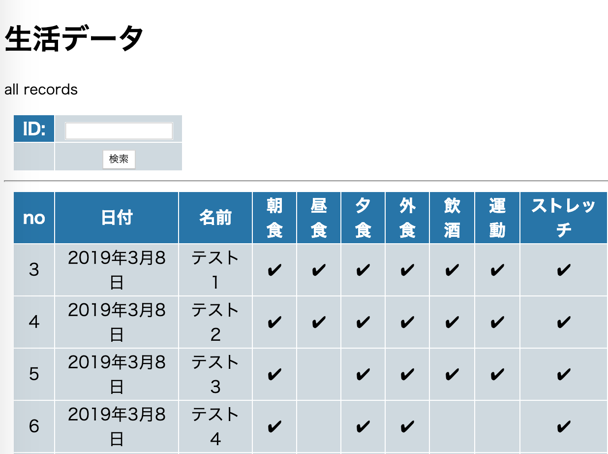
にアクセスしてみましょう。
やってみましょう。このような感じになっていたらOKです。※実際にはyes/noが付いてたらOKです。
メソッドチェーン
特段ここでの用途はないですが、
objects属性でメソッドチェーンを使えば表示するものを制限できます。先ほどのgetのように、valuesというものを使えば、特定の要素だけ取り出すこともできます。また詳細は割愛しますが、メソッドにはcountやfirstなどの便利なものも用意されています。views.pyfrom django.shortcuts import render from django.http import HttpResponse from .models import Touroku from .forms import KenkoForm def index(request): params = { 'title':'生活データ', 'msg':'all records', 'form':KenkoForm(), 'data':[], } if (request.method =='POST'): nametxt = request.POST['name'] item = Touroku.objects.get(name = nametxt) params['data'] = [item] params['form'] = KenkoForm(request.POST) else: params['data'] = Touroku.objects.values("id","name")#ここ return render(request, 'kenko/index.html', params)この記事はここまで
- 投稿日:2019-03-10T19:57:21+09:00
Python手遊び(計画倒れ:GridSearchCV best parameter 少しだけnumpyあり)
この記事、何?
前回記事を深めるつもり・・・だったんだけど、ほとんど深まらなかった。
再利用するかもしれないのでいったん挙げておこうかと。前回記事
■Python機械学習手遊び(GridSearchCVミニマムコード)
https://qiita.com/siinai/items/1aae9462d5e0c9c57344やりたかったこと
f(x, y, z) = ax + by + cz + k + rand()
f(x, y, z) = ax^2 + bx + cy + dz + k + rand()
f(x, y, z) = ax^2 + bx + cy^2 + dy + ez + k + rand()とかいくつか作って、いくつかの予測アルゴリズムを用意して、それぞれにパラメータを与えて試そうかと思った。
こんな感じ。for X, y in dataset: for models, parameter in list: ....ただ、データをまとめようとする時点で迷走してしまって、どれもこれも似たような結果ばかりで・・・
やっぱ駄目ですね。
あまりちゃんとはわかっていないことをわかったつもりで、その「確認」のコーディングをすると。
とりあえずできたところまで上げてコードサンプルにしておこうかと。
全く初めてだと、numpyの列の選択とかも惑う感じなので。。。#31-01.py from sklearn.cross_decomposition import PLSRegression from sklearn.svm import SVR from sklearn.model_selection import GridSearchCV import numpy as np def get_filepath(): return '26-11.txt' def load_data(file): tmp = np.loadtxt(file, delimiter='\t', skiprows=1) X = tmp[:,1:] Y = tmp[:,0:1] return X, Y resultlist = [] def get_model_params(model_flg): if modelflg == 0: modelname = 'PLS' model = PLSRegression() params = [{'n_components':(1, 2, 3)}] raven_flg = False else: modelname = 'SVR' model = SVR() params = [{'kernel':('linear', 'rbf')}] raven_flg = True return modelname, model, params, raven_flg for modelflg in range(2): file = get_filepath() X, Y = load_data(file) modelname, model, params, raven_flg = get_model_params(modelflg) if raven_flg: Y = np.ravel(Y) clf = GridSearchCV(model, params) clf.fit(X, Y) resultlist.append((file, modelname, clf.best_params_, clf.best_score_)) print('----------------------------------------------------------') for result in resultlist: print(result)---------------------------------------------------------- ('26-11.txt', 'PLS', {'n_components': 3}, 0.9999995659126992) ('26-11.txt', 'SVR', {'kernel': 'linear'}, 0.9999995686274493)いや0.9999..って。
乱数強くしすぎるとなんかおかしくなるし・・・ひとまず、書き方自体はわかったので、次は別なことやってみます。
やっぱり、求めたいと思うものをちゃんと定めないと、「やってみた」を超えられない。
意味のある記事にならない。。。
- 投稿日:2019-03-10T19:44:00+09:00
selenium動作用の基底クラスの例を作ってみました
selenium動作用の基底クラス 利用例
概要
以前の記事のクラスを使った例を作ってみました。
seleniumのテスト用のサイトを使用しています。今回は旧サイトを対象にしています。必要なもの
- python 3.7.2
ライブラリとして
- selenium
- numpy
- pandas
- openpyxl
- xlrd
ブラウザは
- Chrome
を使用しています。
公開場所
githubで公開しいます。
使い方
data/予約データ.xlsxに各入力内容に応じて値を入れてください。
- 日付についてはランダムで入るように指定しているので固定したい場合は修正してください。
seleniumTestSite1を実行します。- 終了するのを待ちます。
screenShot/reserveに結果は出力されます。内容の説明
data/予約データ.xlsxの一行ずつ登録を行っていきます。一つのクラスにまとめているが、必要に応じてクラスを分けるなど対応を行います。data/予約データ.xlsxにデータを登録すればまとめて入力できます。CSVなどによる一括登録ができず画面からの入力のみという場合に業務効率化のきっかけにできれば- アラートダイアログに関しては基底クラスに定義していませんが今後定義するかも・・・
- 実際にはこの機能を応用して勤務表の入力やとあるシステムの業務支援として使っています。
- logの設定など見よう見まねでやっているのでベストプラクティスではないかもしれません・・・
- 投稿日:2019-03-10T19:27:57+09:00
Google Cloud Speech-to-Text API を使った複数のチャンネルを含む音声の文字起こし
目的
rebuildfm の Miyagawa さんがGoogle の Cloud Speech-to-Text API を用いてマルチチャンネル音声の文字起こし(コードはこちら)をされていたので、以前自身で書いたブログ(Google Cloud Speech API を使った音声の文字起こし手順)を参考にマルチチャンネル音声の文字起こしにトライ してみました。
Google Cloud-to-Speech マルチチャンネルで 1/2 わけて transcribe するのできた。チャンネルごとに書き出して sox -M でマージ、あとは チャンネル数指定してあげるだけでできた。2ch だったらL/R でやるのでもいいのかも。
— Tatsuhiko Miyagawa (@miyagawa) 2019年2月22日
ただチャンネルごとに書き出すのちょっと面倒。 pic.twitter.com/EtqtNW47f5
事前準備
- 先の記事(Google Cloud Speech API を使った音声の文字起こし手順) の事前準備は実施済みとします
- マルチチャンネル音声データは Google Cloud Platform リポジトリの commercial_stereo.wav をローカルPCにダウンロードしておきます(一応 こちら にも置いておきます)。
手順
0. 準備
先の記事(Google Cloud Speech API を使った音声の文字起こし手順)の手順1 ~ 5 とまで実施し、上記の commercial_stereo.wav を GCP のストレージにアップロードします。
また今回利用するマルチチャンネル音声の文字起こしには、Cloud Speech-to-Text API のベータ版の利用が必要となるため、下記コマンドで Google Cloud Shell上 google-cloud-speech をアップグレードしておきます。
GoogleCloudShell上でgoogle-cloud-speechアップグレードsudo pip install --upgrade google-cloud-speech1. マルチチャンネル音声向けの文字起こしPythonスクリプトの作成
Google Cloud Shell上で文字起こし実行用のPythonスクリプトを作成します。
Pythonファイル編集コマンド(エディタは好きに)$ nano transcribe.py文字起こし用のPythonスクリプト(英語音声用):
multichannel_transcribe.py# !/usr/bin/env python # coding: utf-8 import argparse import io import sys import codecs import datetime import locale def transcribe_gcs(gcs_uri): from google.cloud import speech_v1p1beta1 as speech from google.cloud.speech_v1p1beta1 import enums from google.cloud.speech_v1p1beta1 import types client = speech.SpeechClient() audio = types.RecognitionAudio(uri=gcs_uri) config = types.RecognitionConfig( sample_rate_hertz=44100, encoding=enums.RecognitionConfig.AudioEncoding.LINEAR16, language_code='en-US', audio_channel_count=2, enable_separate_recognition_per_channel=True) operation = client.long_running_recognize(config, audio) print('Waiting for operation to complete...') operationResult = operation.result() d = datetime.datetime.today() today = d.strftime("%Y%m%d-%H%M%S") fout = codecs.open('output{}.txt'.format(today), 'a', 'shift_jis') for result in operationResult.results: for alternative in result.alternatives: fout.write(u'ChannelTag: {}\n'.format(result.channel_tag)) fout.write(u'Transcript: {}\n'.format(alternative.transcript)) fout.close() if __name__ == '__main__': parser = argparse.ArgumentParser( description=__doc__, formatter_class=argparse.RawDescriptionHelpFormatter) parser.add_argument( 'path', help='GCS path for audio file to be recognized') args = parser.parse_args() transcribe_gcs(args.path)ポイントとしては下記3点です:
- マルチチャンネル音声認識の設定として、マルチチャンネル音声のチャンネル数(今回の音源は2チャンネル)の設定、チャンネルごとの音声認識フラグを True にします。
multichannel_transcribe.py(抜粋)audio_channel_count=2, enable_separate_recognition_per_channel=True
- チャンネルごとに分けてテキスト書き出しをします。
multichannel_transcribe.py(抜粋)for result in operationResult.results: for alternative in result.alternatives: fout.write(u'ChannelTag: {}\n'.format(result.channel_tag)) fout.write(u'Transcript: {}\n'.format(alternative.transcript))
- 今回新機能利用のためCloud Speech-to-Text APIベータ版をインポートしています(将来的に正規版に組み込まれた場合は下記正規版のインポートへと記述を変更する必要があると思われます)。
multichannel_transcribe.py(抜粋)from google.cloud import speech_v1p1beta1 as speech from google.cloud.speech_v1p1beta1 import enums from google.cloud.speech_v1p1beta1 import typesまた、日本語の文字起こしをしたい場合は下記1行を修正します:
language_code='en-US')↓
language_code='ja-JP')2. マルチチャンネル音声文字起こしの実行
Google Cloud Console 上で下記コマンドにて文字起こしを実行します。
$ python multichannel_transcribe.py gs://バケット名/音声データ名.wav3. 結果
今回注目したいのが、2人の会話(お店にChromecast を買いに来た人とその店員との会話)が分離された形でチャンネルタグ1 とチャンネルタグ2 として音声認識できている という点です。
これまでの音声ファイルからの文字起こしではこうしたチャンネルごとに分けられずテキストが出力されていました。
今回Cloud Speech-to-Text APIベータ版のマルチチャンネル音声の文字起こし機能を利用することで、電話の受け答えのような複数のチャンネルを含んだ音声についてチャンネルを分けた形で文字起こしができそうという手ごたえを得られました。
ChannelTag: 1
Transcript: hi I'd like to buy a Chromecast I was wondering whether you could help me with that
ChannelTag: 2
Transcript: certainly which color would you like we have blue black and red
ChannelTag: 1
Transcript:  let's go with the black one
ChannelTag: 2
Transcript:  would you like the new Chromecast Ultra model or the regular Chromecast
ChannelTag: 1
Transcript:  regular Chromecast is fine thank you
ChannelTag: 2
Transcript:  okay sure would you like to ship it regular or Express
ChannelTag: 1
Transcript:  express please
ChannelTag: 2
Transcript:  terrific it's on the way thank you
ChannelTag: 1
Transcript:  thank you very much bye
参考
- https://twitter.com/miyagawa/status/1098815809701347328
- https://gist.github.com/miyagawa/7624f237f103554fdfbdad44f8857355
- https://cloud.google.com/speech-to-text/docs/multi-channel?hl=ja#speech-multi-channel-python
- https://stackoverflow.com/questions/50773013/importerror-cannot-import-name-speech-v1p1beta1
所感
- 今回本当は rebuildfm #131 の「年の割に無責任 」 の回(自分の好きな回)をチャンネルを分けた形で文字起こししてみたいと考えてトライしたのがきっかけでした。
- しかし、結果として Podcastサイトの mp3 をそのままダウンロードした場合、音源データ自体が複数チャンネル情報を含んでいなかったため、上記 Python スクリプト実行時に「設定されらチャンネル数が間違っている」という意味のエラーで複数のチャンネル音声の文字起こしはできませんでした。。( ;∀;)
- そのため、適用範囲としては複数人の声が入った音声データではなく、あくまで音声データ自体がマルチチャンネル音声である必要がある 点、注意点として強調しておきたいと感じました。


- 投稿日:2019-03-10T19:13:26+09:00
[深層学習]webカメラで顔認識して、linebotで報告するシステムをつくった。
はじめに
私が所属しているサークルでは、部屋の出入りをいちいちLINEとslackで報告しなくてはならず、これがめんどい。。。。
ならば、監視カメラ的な物をつくってLINEbotとslackbotに代わりに報告してもらおう!というのがコレを作った動機です。流れは、
1.webカメラを起動する
2.カメラで顔を認識したら、顔の部分だけをトリミングして保存
3.保存した画像を学習済みモデルに通して分類する
4.分類結果をLINE,slackbotからメッセージとして送信する
という感じです。サークルメンバー10人の顔を見分けたい!!
目次
1.環境
2.画像収集
3.画像の水増し
3.転移学習
4.webカメラの起動・LINE,slackとの連携
5.終わりに環境
・python 3.6.5
・opencv-python 3.4.4.19
・Keras 2.2.4
・Flask 1.0.2
・line-bot-sdk 1.8.0
・slackbot 0.5.3画像収集
画像はLINEグループのアルバムから丸ごともってきました。
学習データ用に、これらの画像から顔だけを切り出していきます!
学習済みの検出器をこちらから持ってきて、face_cut.pyと同じ階層においておきました。face_cut.pyimport cv2 import glob import numpy as np model = "./models/haarcascade_frontalface_alt.xml" faceCascade = cv2.CascadeClassifier(model)#顔検出器を生成 PHOTOS_PATH = "./input_done" SAVE_PATH = "./detected_faces" files = glob.glob(PHOTOS_PATH + "/*.jpg") detect_count= 0 undetect_count= 0 read_count = 0 for i,file in enumerate(files): img = cv2.imread(file)#第二引数に0指定しろよ img = cv2.cvtColor(img, cv2.COLOR_RGB2GRAY) h, w = img.shape[:2] img = cv2.resize(img, (w,h))#結局リサイズしてない。 face = faceCascade.detectMultiScale(img)#顔として認識した正方形の左上の座標がx,yに、横、縦幅がw,hに格納されている read_count += 1 if len(face)>0:#顔を認識したら、 for rect in face:#認識したすべての顔を切り出す cv2.imwrite(SAVE_PATH + "/" +str(read_count) + "_" + str(detect_count) +".jpg", img[rect[1]:rect[1] + rect[3], rect[0]:rect[0] + rect[2]]) detect_count += 1 print("detect!",detect_count) else: undetect_count += 1 print("undetect...", undetect_count) print("detect_count", detect_count) print("undetect_count", undetect_count)
PHOTOS_PATHで指定したフォルダの画像を読み込み、切り出した画像はSAVE_PATHで指定したフォルダに保存します。この後、画像を使いやすいようにクラス(人物)ごとにフォルダに分類しました。この作業で6時間くらいかかった。。。
......さあ、各クラス150枚準備できました!
画像の水増し
さっそく学習!...といきたいのですが、これだけでは足りないのでトレーニングデータを水増ししていきます!
トレーニングデータには120枚をあてました。それぞれの画像に対して左右反転、コントラスト調整、平滑化、γ変換をして2^4倍に増やします。
この際、水増しをするのはトレーニングデータのみにします。face_aug.pyimport cv2 import os,glob import numpy as np from sklearn import model_selection #クラスごとのフォルダ名をリストにまとめる classes = ["member1","menber2","member3","member4","member5","member6","member7","member8","member9","member10","others"] num_classes = len(classes) image_size = 50 X_train = [] X_test = [] y_train = [] y_test = [] #----------------------------------------------------------- #~水増しする関数のみなさん~ #左右反転 def flip(img): #第二引数を正でy軸対象 flip_images = cv2.flip(img, 1) return flip_images #コントラスト def cont(img): #ルックアップテーブルの生成 min_table=50 max_table=205 diff_table=max_table - min_table LUT_HC = np.arange(256, dtype = "uint8") #ハイコントラストLUT作成 for i in range(0, min_table): LUT_HC[i] = 0 for i in range(min_table, max_table): LUT_HC[i] = 255 * (i - min_table) / diff_table for i in range(max_table, 255): LUT_HC[i] = 255 #変換 #cv2.LUTで適用 high_cont_imgs = cv2.LUT(img, LUT_HC) return high_cont_imgs #ぼかし def blur(img): blur_images = cv2.GaussianBlur(img, (5, 5), 0) return blur_images #γ変換 def gamma(img): # ガンマ変換ルックアップテーブル gamma1 = 0.75 LUT_G1 = np.arange(256, dtype="uint8") for i in range(256): LUT_G1[i] = 255 * pow(float(i) / 255, 1.0 / gamma1) #変換 gamma1_images = cv2.LUT(img, LUT_G1) return gamma1_images #----------------------------------------------------------------- for index, classlabel in enumerate(classes): photos_dir = "./" + classlabel files = glob.glob(photos_dir + "/*.jpg") for i,file in enumerate(files): if i >= 150: #ラベルごとの画像の枚数をそろえる break img = cv2.imread(file) img = cv2.resize(img, (image_size,image_size)) if i < 30: #この番号以下の写真のデータはテスト用になる data = np.asarray(img) X_test.append(data) y_test.append(index) else: #それ以外はトレーニング用になる #1枚の画像ずつ処理する images = [img] images.extend(list(map(flip, images)))#倍倍に増えていく~ images.extend(list(map(cont, images))) images.extend(list(map(blur, images))) images.extend(list(map(gamma, images))) for _ in range(len(images)):#imagesの枚数分だけ正解ラベルを作成 y_train.append(index) #処理した全ての画像を格納する X_train.extend(images) print(classlabel , "done!") X_train = np.array(X_train)#nparrayに変換する X_test = np.array(X_test) y_train = np.array(y_train) y_test = np.array(y_test) xy = (X_train,X_test,y_train,y_test)#これらをxyにまとめ、 np.save("./face_aug.npy", xy)#画像データを保存する #ちゃんとデータができているか確認した X_train, X_test, y_train, y_test = np.load("face_aug.npy") print(len(X_train),len(X_test),len(y_train),len(y_test)) for i in range(len(classes)): count = 0 for j in range(len(y_train)): if y_train[j] == i: count += 1 print(count)各クラス約2000枚のデータがそろったので、いよいよ転移学習させていきましょう?
VGG16で転移学習させる
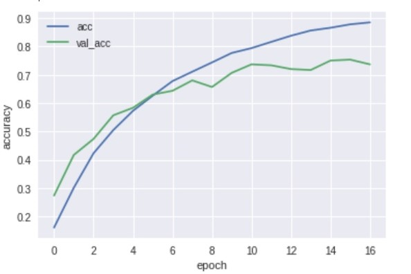
vgg16.pyfrom keras import optimizers from keras.applications.vgg16 import VGG16 from keras.datasets import cifar10 from keras.layers import Dense, Dropout, Flatten, Input, BatchNormalization, Activation from keras.models import Model, Sequential from keras.callbacks import EarlyStopping from keras.utils import plot_model, np_utils import matplotlib.pyplot as plt import numpy as np %matplotlib inline classes = ["member1","menber2","member3","member4","member5","member6","member7","member8","member9","member10","others"] num_classes = len(classes) epochs=20 batch_size=64 X_train, X_test, y_train, y_test = np.load("face_aug.npy") X_train = X_train.astype("float") / 255 #X_trainの各チャンネルの値は0~255だがそれを255で割ることですべての値を0~1にする(正規化) X_test = X_test.astype("float") / 255 y_train = np_utils.to_categorical(y_train, num_classes) #one_hotベクトルに変換 y_test = np_utils.to_categorical(y_test, num_classes) input_tensor = Input(shape=(50, 50, 1)) vgg16 = VGG16(include_top=False, weights='imagenet', input_tensor=input_tensor) top_model = Sequential() top_model.add(Flatten(input_shape=vgg16.output_shape[1:])) #top_model.add(Dense(128)) #top_model.add(BatchNormalization()) #top_model.add(Activation('sigmoid')) #top_model.add(Dropout(0.5)) #top_model.add(Dense(64)) #top_model.add(BatchNormalization()) #top_model.add(Activation('sigmoid')) #top_model.add(Dropout(0.5)) top_model.add(Dense(32)) #top_model.add(BatchNormalization()) top_model.add(Activation('sigmoid')) #top_model.add(Dropout(0.5)) top_model.add(Dense(num_classes, activation="softmax")) model = Model(inputs=vgg16.input, outputs=top_model(vgg16.output)) for layer in model.layers[:6]:#VGGの層の重みの固定を調整する layer.trainable = False model.compile(optimizer=optimizers.SGD (lr=1e-4, momentum=0.9),loss='categorical_crossentropy', metrics=['accuracy']) es = EarlyStopping(monitor='val_loss', patience=0, verbose=0, mode='min')#バリデーションデータ(テストデータ)の損失関数の値が大きくなると早期終了する history = model.fit(X_train, y_train, validation_data=(X_test, y_test), batch_size=batch_size, epochs=epochs, callbacks=[es]) model.save("faces.h5") #モデルの評価 scores = model.evaluate(X_test, y_test, verbose=1) print('Test loss: ', scores[0]) print('Test accuracy: ', scores[1]) print() #学習曲線の表示 plt.plot(history.history['acc'], label='acc', ls='-') plt.plot(history.history['val_acc'], label='val_acc', ls='-') plt.ylabel('accuracy') plt.xlabel('epoch') plt.legend(loc='best') plt.show()結果は75%くらい。
グラフ見た感じもっと精度あげられそう。
実用化するなら95%くらい欲しいけど、妥協しました。。
いろんなサイズのモデルで学習させてみましたが、1番精度が良かったのはごく小さなモデルでした。
考察してみた
・今回は50x50にリサイズしたが、元画像がそれよりも小さい画像があった。そのため、かなりぼやけてしまい上手く学習できなかったのではないか。
・今回はサークルメンバー以外の人も分類できるように、othersクラスを設けた。このクラスだけ異なる多数の人の顔で学習させたので、上手く重みの調整ができなかったのかもしれない。
・重みを固定するVGGの層を減らした方が精度がよかった。初期の層でよりプリミティブな特徴を捉え、残りの層で今回扱ったデータ特有の特徴を捉えたためだろう。こういう結果が出たのは、imagenetが人の顔を含んでいないためだろうか。
webカメラの起動・LINEとslackとの連携
いよいよ、先ほど作成したモデルと、LINEとslackとの連携部分を書いていきます!
長々とディープラーニングについて書いてきましたが、メインはこれからですね!
came.pyでwebカメラを起動して、顔を認識したらdetect_pushモジュールを呼び出してLINEbotとslackbotからメッセージを送っています。(以前は
subprocess.check_call()を使っていました。モジュール化すると見やすいですね。)came.pyimport cv2 import numpy as np from keras.models import load_model from detect_push import detectFace, pushToLine, pushToSlack import time SAVE_PATH = "./input/face.jpg" model = load_model('faces.h5') face_cascade = cv2.CascadeClassifier('./models/haarcascade_frontalface_default.xml') cap = cv2.VideoCapture(0)#webカメラをキャプチャーする while True: ret, img = cap.read() img = cv2.flip(img, 1)#反転 gray = cv2.cvtColor(img, cv2.COLOR_BGR2GRAY)#グレースケール化 cv2.imshow("img",img) faces = face_cascade.detectMultiScale(gray, 1.9, 5) if len(face)>0: for rect in face: cv2.imwrite(SAVE_PATH, img[rect[1]:rect[1] + rect[3], rect[0]:rect[0] + rect[2]]) print("recognize face !!") member = detectFace(SAVE_PATH, model)#上で保存した画像を読み込み、モデルでの予測結果をmemberに代入 pushToLine(member)#予測結果を受け取り、LINEbotから送信 pushToSlack(member)#予測結果を受け取り、slackbotから送信 time.sleep(10) if cv2.waitKey(30) == 27:#Escキーを押すとbreak break # キャプチャをリリースして、ウィンドウをすべて閉じる cap.release() cv2.destroyAllWindows()detect_push.pyimport os import tensorflow as tf import cv2 import numpy as np from linebot import LineBotApi from linebot.models import TextSendMessage, ImageSendMessage from linebot.exceptions import LineBotApiError from slackbot.slackclient import SlackClient def detectFace(filepath, model):#指定されたパスの画像を読み込んで,予測結果を返す image = cv2.imread(filepath) image = cv2.resize(image,(50,50)) data = np.expand_dims(image, axis=0) result = model.predict(data) predicted = result.argmax() members = ["member1","member2","member3","member4","member5","member6","member7","member8","member9","member10","others"] return members[predicted] def pushToLine(member):#LINEbotからメッセージを送信する channel_access_token = os.getenv('LINE_CHANNEL_ACCESS_TOKEN', None)#環境変数に設定したchannel_access_tokenを取得 line_bot_api = LineBotApi(channel_access_token) try: line_bot_api.push_message("メッセージを送信したいトークルームのid", TextSendMessage(text = member + "が開けました")) except LineBotApiError as e: # error handle ... def pushToSlack(member):#slackbotからメッセージを送信する #slackclientのインスタンスを作成 bot = SlackClient("slackbotのid") bot.send_message("メッセージを送信したいチャンネル名", member + "が開けました")これだけの記述でbotからメッセージが送れる!!!
各アカウント登録は最後にリンクを張っておくので、そのサイトを参考にしてみてください。
公式ドキュメントを見た感じ、LINEbotでもっといろんなことができそうですね...!まとめ
kerasでめちゃめちゃ簡単にモデルが作れて、転移学習であまり考えずにそこそこの精度がでる。
ただ学習データの準備がものすごく大変です。。。
LINEbotもslackbotも簡単に作れたので、他に面白いbotを作ったら紹介したいですね!
参考にしたサイト
Kerasでアニメ 「けいおん!」を画像認識させてみた
openCVで複数画像ファイルから顔検出をして切り出し保存
Messaging APIを利用するには-LINE Developers
Pythonを使ったSlackBotの作成方法
- 投稿日:2019-03-10T19:13:26+09:00
[深層学習]webカメラで顔認識して、LINEbotで報告するシステムをつくった。
はじめに
私が所属しているサークルでは、部屋の出入りをいちいちLINEとslackで報告しなくてはならず、これがめんどい。。。。
ならば、監視カメラ的な物をつくってLINEbotとslackbotに代わりに報告してもらおう!というのがコレを作った動機です。流れは、
1.webカメラを起動する
2.カメラで顔を認識したら、顔の部分だけをトリミングして保存
3.保存した画像を学習済みモデルに通して分類する
4.分類結果をLINE,slackbotからメッセージとして送信する
という感じです。サークルメンバー10人の顔を見分けたい!!
目次
1.環境
2.画像収集
3.画像の水増し
3.転移学習
4.webカメラの起動・LINE,slackとの連携
5.終わりに環境
・python 3.6.5
・opencv-python 3.4.4.19
・Keras 2.2.4
・Flask 1.0.2
・line-bot-sdk 1.8.0
・slackbot 0.5.3画像収集
画像はLINEグループのアルバムから丸ごともってきました。
学習データ用に、これらの画像から顔だけを切り出していきます!
学習済みの検出器をこちらから持ってきて、face_cut.pyと同じ階層においておきました。face_cut.pyimport cv2 import glob import numpy as np model = "./models/haarcascade_frontalface_alt.xml" faceCascade = cv2.CascadeClassifier(model)#顔検出器を生成 PHOTOS_PATH = "./input_done" SAVE_PATH = "./detected_faces" files = glob.glob(PHOTOS_PATH + "/*.jpg") detect_count= 0 undetect_count= 0 read_count = 0 for i,file in enumerate(files): img = cv2.imread(file)#第二引数に0指定しろよ img = cv2.cvtColor(img, cv2.COLOR_RGB2GRAY) h, w = img.shape[:2] img = cv2.resize(img, (w,h))#結局リサイズしてない。 face = faceCascade.detectMultiScale(img)#顔として認識した正方形の左上の座標がx,yに、横、縦幅がw,hに格納されている read_count += 1 if len(face)>0:#顔を認識したら、 for rect in face:#認識したすべての顔を切り出す cv2.imwrite(SAVE_PATH + "/" +str(read_count) + "_" + str(detect_count) +".jpg", img[rect[1]:rect[1] + rect[3], rect[0]:rect[0] + rect[2]]) detect_count += 1 print("detect!",detect_count) else: undetect_count += 1 print("undetect...", undetect_count) print("detect_count", detect_count) print("undetect_count", undetect_count)
PHOTOS_PATHで指定したフォルダの画像を読み込み、切り出した画像はSAVE_PATHで指定したフォルダに保存します。この後、画像を使いやすいようにクラス(人物)ごとにフォルダに分類しました。この作業で6時間くらいかかった。。。
......さあ、各クラス150枚準備できました!
画像の水増し
さっそく学習!...といきたいのですが、これだけでは足りないのでトレーニングデータを水増ししていきます!
トレーニングデータには120枚をあてました。それぞれの画像に対して左右反転、コントラスト調整、平滑化、γ変換をして2^4倍に増やします。
この際、水増しをするのはトレーニングデータのみにします。face_aug.pyimport cv2 import os,glob import numpy as np from sklearn import model_selection #クラスごとのフォルダ名をリストにまとめる classes = ["member1","menber2","member3","member4","member5","member6","member7","member8","member9","member10","others"] num_classes = len(classes) image_size = 50 X_train = [] X_test = [] y_train = [] y_test = [] #----------------------------------------------------------- #~水増しする関数のみなさん~ #左右反転 def flip(img): #第二引数を正でy軸対象 flip_images = cv2.flip(img, 1) return flip_images #コントラスト def cont(img): #ルックアップテーブルの生成 min_table=50 max_table=205 diff_table=max_table - min_table LUT_HC = np.arange(256, dtype = "uint8") #ハイコントラストLUT作成 for i in range(0, min_table): LUT_HC[i] = 0 for i in range(min_table, max_table): LUT_HC[i] = 255 * (i - min_table) / diff_table for i in range(max_table, 255): LUT_HC[i] = 255 #変換 #cv2.LUTで適用 high_cont_imgs = cv2.LUT(img, LUT_HC) return high_cont_imgs #ぼかし def blur(img): blur_images = cv2.GaussianBlur(img, (5, 5), 0) return blur_images #γ変換 def gamma(img): # ガンマ変換ルックアップテーブル gamma1 = 0.75 LUT_G1 = np.arange(256, dtype="uint8") for i in range(256): LUT_G1[i] = 255 * pow(float(i) / 255, 1.0 / gamma1) #変換 gamma1_images = cv2.LUT(img, LUT_G1) return gamma1_images #----------------------------------------------------------------- for index, classlabel in enumerate(classes): photos_dir = "./" + classlabel files = glob.glob(photos_dir + "/*.jpg") for i,file in enumerate(files): if i >= 150: #ラベルごとの画像の枚数をそろえる break img = cv2.imread(file) img = cv2.resize(img, (image_size,image_size)) if i < 30: #この番号以下の写真のデータはテスト用になる data = np.asarray(img) X_test.append(data) y_test.append(index) else: #それ以外はトレーニング用になる #1枚の画像ずつ処理する images = [img] images.extend(list(map(flip, images)))#倍倍に増えていく~ images.extend(list(map(cont, images))) images.extend(list(map(blur, images))) images.extend(list(map(gamma, images))) for _ in range(len(images)):#imagesの枚数分だけ正解ラベルを作成 y_train.append(index) #処理した全ての画像を格納する X_train.extend(images) print(classlabel , "done!") X_train = np.array(X_train)#nparrayに変換する X_test = np.array(X_test) y_train = np.array(y_train) y_test = np.array(y_test) xy = (X_train,X_test,y_train,y_test)#これらをxyにまとめ、 np.save("./face_aug.npy", xy)#画像データを保存する #ちゃんとデータができているか確認した X_train, X_test, y_train, y_test = np.load("face_aug.npy") print(len(X_train),len(X_test),len(y_train),len(y_test)) for i in range(len(classes)): count = 0 for j in range(len(y_train)): if y_train[j] == i: count += 1 print(count)各クラス約2000枚のデータがそろったので、いよいよ転移学習させていきましょう?
VGG16で転移学習させる
vgg16.pyfrom keras import optimizers from keras.applications.vgg16 import VGG16 from keras.datasets import cifar10 from keras.layers import Dense, Dropout, Flatten, Input, BatchNormalization, Activation from keras.models import Model, Sequential from keras.callbacks import EarlyStopping from keras.utils import plot_model, np_utils import matplotlib.pyplot as plt import numpy as np %matplotlib inline classes = ["member1","menber2","member3","member4","member5","member6","member7","member8","member9","member10","others"] num_classes = len(classes) epochs=20 batch_size=64 X_train, X_test, y_train, y_test = np.load("face_aug.npy") X_train = X_train.astype("float") / 255 #X_trainの各チャンネルの値は0~255だがそれを255で割ることですべての値を0~1にする(正規化) X_test = X_test.astype("float") / 255 y_train = np_utils.to_categorical(y_train, num_classes) #one_hotベクトルに変換 y_test = np_utils.to_categorical(y_test, num_classes) input_tensor = Input(shape=(50, 50, 1)) vgg16 = VGG16(include_top=False, weights='imagenet', input_tensor=input_tensor) top_model = Sequential() top_model.add(Flatten(input_shape=vgg16.output_shape[1:])) #top_model.add(Dense(128)) #top_model.add(BatchNormalization()) #top_model.add(Activation('sigmoid')) #top_model.add(Dropout(0.5)) #top_model.add(Dense(64)) #top_model.add(BatchNormalization()) #top_model.add(Activation('sigmoid')) #top_model.add(Dropout(0.5)) top_model.add(Dense(32)) #top_model.add(BatchNormalization()) top_model.add(Activation('sigmoid')) #top_model.add(Dropout(0.5)) top_model.add(Dense(num_classes, activation="softmax")) model = Model(inputs=vgg16.input, outputs=top_model(vgg16.output)) for layer in model.layers[:6]:#VGGの層の重みの固定を調整する layer.trainable = False model.compile(optimizer=optimizers.SGD (lr=1e-4, momentum=0.9),loss='categorical_crossentropy', metrics=['accuracy']) es = EarlyStopping(monitor='val_loss', patience=0, verbose=0, mode='min')#バリデーションデータ(テストデータ)の損失関数の値が大きくなると早期終了する history = model.fit(X_train, y_train, validation_data=(X_test, y_test), batch_size=batch_size, epochs=epochs, callbacks=[es]) model.save("faces.h5") #モデルの評価 scores = model.evaluate(X_test, y_test, verbose=1) print('Test loss: ', scores[0]) print('Test accuracy: ', scores[1]) print() #学習曲線の表示 plt.plot(history.history['acc'], label='acc', ls='-') plt.plot(history.history['val_acc'], label='val_acc', ls='-') plt.ylabel('accuracy') plt.xlabel('epoch') plt.legend(loc='best') plt.show()結果は75%くらい。
グラフ見た感じもっと精度あげられそう。
実用化するなら95%くらい欲しいけど、妥協しました。。
いろんなサイズのモデルで学習させてみましたが、1番精度が良かったのはごく小さなモデルでした。
考察してみた
・今回は50x50にリサイズしたが、元画像がそれよりも小さい画像があった。そのため、かなりぼやけてしまい上手く学習できなかったのではないか。
・今回はサークルメンバー以外の人も分類できるように、othersクラスを設けた。このクラスだけ異なる多数の人の顔で学習させたので、上手く重みの調整ができなかったのかもしれない。
・重みを固定するVGGの層を減らした方が精度がよかった。初期の層でよりプリミティブな特徴を捉え、残りの層で今回扱ったデータ特有の特徴を捉えたためだろう。こういう結果が出たのは、imagenetが人の顔を含んでいないためだろうか。
webカメラの起動・LINEとslackとの連携
いよいよ、先ほど作成したモデルと、LINEとslackとの連携部分を書いていきます!
長々とディープラーニングについて書いてきましたが、メインはこれからですね!
came.pyでwebカメラを起動して、顔を認識したらdetect_pushモジュールを呼び出してLINEbotとslackbotからメッセージを送っています。(以前は
subprocess.check_call()を使っていました。モジュール化すると見やすいですね。)came.pyimport cv2 import numpy as np from keras.models import load_model from detect_push import detectFace, pushToLine, pushToSlack import time SAVE_PATH = "./input/face.jpg" model = load_model('faces.h5') face_cascade = cv2.CascadeClassifier('./models/haarcascade_frontalface_default.xml') cap = cv2.VideoCapture(0)#webカメラをキャプチャーする while True: ret, img = cap.read() img = cv2.flip(img, 1)#反転 gray = cv2.cvtColor(img, cv2.COLOR_BGR2GRAY)#グレースケール化 cv2.imshow("img",img) faces = face_cascade.detectMultiScale(gray, 1.9, 5) if len(face)>0: for rect in face: cv2.imwrite(SAVE_PATH, img[rect[1]:rect[1] + rect[3], rect[0]:rect[0] + rect[2]]) print("recognize face !!") member = detectFace(SAVE_PATH, model)#上で保存した画像を読み込み、モデルでの予測結果をmemberに代入 pushToLine(member)#予測結果を受け取り、LINEbotから送信 pushToSlack(member)#予測結果を受け取り、slackbotから送信 time.sleep(10) if cv2.waitKey(30) == 27:#Escキーを押すとbreak break # キャプチャをリリースして、ウィンドウをすべて閉じる cap.release() cv2.destroyAllWindows()detect_push.pyimport os import tensorflow as tf import cv2 import numpy as np from linebot import LineBotApi from linebot.models import TextSendMessage, ImageSendMessage from linebot.exceptions import LineBotApiError from slackbot.slackclient import SlackClient def detectFace(filepath, model):#指定されたパスの画像を読み込んで,予測結果を返す image = cv2.imread(filepath) image = cv2.resize(image,(50,50)) data = np.expand_dims(image, axis=0) result = model.predict(data) predicted = result.argmax() members = ["member1","member2","member3","member4","member5","member6","member7","member8","member9","member10","others"] return members[predicted] def pushToLine(member):#LINEbotからメッセージを送信する channel_access_token = os.getenv('LINE_CHANNEL_ACCESS_TOKEN', None)#環境変数に設定したchannel_access_tokenを取得 line_bot_api = LineBotApi(channel_access_token) try: line_bot_api.push_message("メッセージを送信したいトークルームのid", TextSendMessage(text = member + "が開けました")) except LineBotApiError as e: # error handle ... def pushToSlack(member):#slackbotからメッセージを送信する #slackclientのインスタンスを作成 bot = SlackClient("slackbotのid") bot.send_message("メッセージを送信したいチャンネル名", member + "が開けました")これだけの記述でbotからメッセージが送れる!!!
各アカウント登録は最後にリンクを張っておくので、そのサイトを参考にしてみてください。
公式ドキュメントを見た感じ、LINEbotでもっといろんなことができそうですね...!まとめ
kerasでめちゃめちゃ簡単にモデルが作れて、転移学習であまり考えずにそこそこの精度がでる。
ただ学習データの準備がものすごく大変です。。。
LINEbotもslackbotも簡単に作れたので、他に面白いbotを作ったら紹介したいですね!
参考にしたサイト
Kerasでアニメ 「けいおん!」を画像認識させてみた
openCVで複数画像ファイルから顔検出をして切り出し保存
Messaging APIを利用するには-LINE Developers
Pythonを使ったSlackBotの作成方法
- 投稿日:2019-03-10T19:07:53+09:00
Python でモジュールごとに logging する。または dictConfig の落とし穴。
Python でちょっと凝ったログの出力をしたい場合 logging というライブラリを使うのが定番です。また設定には dictConfig を使います。ただ後方互換性のために落とし穴があるので、意図しない動作になる時は disable_existing_loggers を False にするのがコツです。と、いうような話題を書きます。
logging には2つの主要な要素 Logger と Handler があります。
基本の使い方
基本の使い方は簡単です。
# 以下の二行はイディオムです。現在のモジュール名が付いた Logger が出来ます。
import logging
logger = logging.getLogger(__name__)

# Logger には debug, info, warning などのメソッドがあるので、重要度に応じて使います。
logger.debug('Debug')
logger.info('Info')
logger.warning('Warning')
この例では Handler が指定されていないので、デフォルトの Handler が使われます。デフォルトの Handler は WARNING 以上のログを stderr に書き込みます。というわけでここでは DEBUG や INFO は無視されて、次のように表示します。
Warnちょっと深入りしますが、デフォルトの動作の実装を見ます。
ライブラリコードを見ると、ここは 「何も Handler が登録されていない時は lastResort を使う」 となっています。
        if (found == 0):
            if lastResort:
                if record.levelno >= lastResort.level:
                    lastResort.handle(record)
lastResort の定義は、「level が WARNING で stderr に出力する StreamHandler」 です。このハンドラは全くカスタマイズ出来ないので、デフォルト動作はオマケと考えるべきです。
_defaultLastResort = _StderrHandler(WARNING)
lastResort = _defaultLastResort
info や debug を表示する。
WARNING 以下のログも表示したい場合は自分で Handler を用意します。(本当は basicConfig でもっと簡単に設定出来ますが、応用が効かないのでここでは触れません。)
import logging
logger = logging.getLogger(__name__)

# ログを stderr に表示する StreamHandler を作る。
handler = logging.StreamHandler()

# logger に StreamHandler を設定する。
logger.addHandler(handler)

# logger の閾値を DEBUG 以上に設定する。
logger.setLevel(logging.DEBUG)

logger.debug('Debug')
logger.info('Info')
logger.warning('Warning')
addHandler()によってデフォルトの lastResort の代わりに指定した Handler を使います。そしてsetLevel()で閾値を設定します。setLevel()は Logger 側にも Handler 側にもあり、両方の条件を満たしたログだけ表示します。Logger 側の閾値のデフォルトは WARNING なので DEBUG を表示したい場合は明示的にsetLevel()する必要があります。Handler 側のデフォルトは NOTSET (閾値なし) なので未設定で良いです。実行結果はこうなります。Debug Info WarnLogger の階層構造
Logger には階層構造があります。
- logging.getLogger(): getLogger を引数無しで呼ぶと root logger が得られる。すべての Logger の親。
- logging.getLogger('parent'): getLogger に引数を指定すると、名前付き logger が返る。通常
logging.getLogger(__name__)を使う。- logging.getLogger('parent.child'): 名前は . で区切った階層構造を持つ。'parent.child' の親は 'parent'。
先程、「Logger の閾値のデフォルトは WARNING」と書いたのは嘘です。正確には:
- Logger の閾値のデフォルトは NOTSET。つまり未設定。この場合親の閾値が使われる。
- logger.getLogger() すなわち root logger の閾値はデフォルトで WARNING。
- よって、Logger の実質的な閾値のデフォルトは WARNING。
この動作を確認するために、
logging.getLogger(__name__)で得られる logger__main__の代わりに root logger を設定しても上記と同じ結果になります。import logging logger = logging.getLogger(__name__) # ログを stderr に表示する StreamHandler を作る。 handler = logging.StreamHandler() # logging.getLogger(__name__) の代わりに root logger に StreamHandler を設定して閾値を DEBUG にする。 logging.getLogger().addHandler(handler) logging.getLogger().setLevel(logging.DEBUG) logger.debug('Debug') logger.info('Info') logger.warning('Warning')モジュールのログを表示
複数のモジュールで出来ているプログラムのログが必要な時に、モジュールを選んで表示したり閾値を変えたくなります。たとえば module.py という名前のモジュールがあるとします。
# module.py
import logging
logger = logging.getLogger(__name__)

def log():
    logger.debug('Debug')
    logger.info('Info')
    logger.warning('Warning')
これ呼び出して、先程と同じように Debug ログを表示してみます。分かりやすいように書式も変更します。
import module
import logging
logger = logging.getLogger(__name__)

# ログを stderr に表示する StreamHandler を作り、書式を設定する。
handler = logging.StreamHandler()
handler.setFormatter(logging.Formatter("%(levelname)s:%(name)s:%(message)s"))

# logger に StreamHandler を設定する。
logger.addHandler(handler)

# logger の閾値を DEBUG 以上に設定する。
logger.setLevel(logging.DEBUG)

logger.debug('Debug')
logger.info('Info')
logger.warning('Warning')

module.log()
残念ながら、Debug ログが表示されたのはメインのスクリプトだけで、
module.log()にはデフォルトの handler が適用されてしまい Debug が表示されません。DEBUG:__main__:Debug INFO:__main__:Info WARNING:__main__:Warning Warningモジュール内の Debug ログも表示したい時は明示的に handler を設定します。
import module
import logging
logger = logging.getLogger(__name__)

# ログを stderr に表示する StreamHandler を作り、書式を設定する。
handler = logging.StreamHandler()
handler.setFormatter(logging.Formatter("%(levelname)s:%(name)s:%(message)s"))

# このスクリプトの logger に先程作った Handler を登録して閾値を DEBUG にする。
logger.addHandler(handler)
logger.setLevel(logging.DEBUG)

# module の logger に先程作った Handler を登録して閾値を DEBUG にする。
logging.getLogger('module').addHandler(handler)
logging.getLogger('module').setLevel(logging.DEBUG)

logger.debug('Debug')
logger.info('Info')
logger.warning('Warning')

module.log()
出力
DEBUG:__main__:Debug
INFO:__main__:Info
WARNING:__main__:Warning
DEBUG:module:Debug
INFO:module:Info
WARNING:module:Warning
モジュールのログを表示 (root logger で手抜き)
もしも利用するモジュール全部のログを同じように表示したいだけなら、root logger で全部まとめて設定出来ます。
import module
import logging
logger = logging.getLogger(__name__)

# 以下の設定は logging.basicConfig(level=logging.DEBUG) と同じです。

# ログを stderr に表示する StreamHandler を作り、書式を設定する。
handler = logging.StreamHandler()
handler.setFormatter(logging.Formatter("%(levelname)s:%(name)s:%(message)s"))

# 各 logger の代わりに root logger を設定する。
logging.getLogger().addHandler(handler)
logging.getLogger().setLevel(logging.DEBUG)

logger.debug('Debug')
logger.info('Info')
logger.warning('Warning')

module.log()
実行結果は上と同様です。
Formatter による書式設定
"%(levelname)s:%(name)s:%(message)s"のような記法で書式設定します。非常に分かりづらいですが、levelnameなどの名前は LogRecord attributes で定義されています。時刻の指定はちょっと特殊で (あとで書く)
dictConfig による設定
このようにすると柔軟にログを設定出来ますが、ややこしくてやってられないと思います。dictConfig というのを使うと多少楽になります。
import logging
import logging.config
import module
import yaml
logger = logging.getLogger(__name__)

logging.config.dictConfig(yaml.load("""
version: 1
formatters:
    default: { format: '%(levelname)s:%(name)s:%(message)s' }
handlers:
    console: { class: logging.StreamHandler, level: DEBUG, formatter: default }
loggers:
    module: { level: DEBUG, handlers: [ console ], }
    __main__: { level: DEBUG, handlers: [ console ], }
"""))

logger.debug('Debug')
logger.info('Info')
logger.warning('Warning')

module.log()
出力
DEBUG:__main__:Debug
INFO:__main__:Info
WARNING:__main__:Warning
DEBUG:module:Debug
INFO:module:Info
WARNING:module:Warning
dictConfig 固有の書き方を覚えないといけないので、python 素の python で地道に書くより簡単かどうかは微妙ですが、dictConfig を使った既存のプロジェクトを使う時や、複雑な設定が必要な時には使うしか無いです。
dictConfig は既存の logger を消してしまう!
ただ、dictConfig には既存の logger を消してしまうという分かりづらい落とし穴があります。例えば上の例をさらにシンプルにして root logger での設定を試みます。
import logging
import logging.config
import module
import yaml
logger = logging.getLogger(__name__)

logging.config.dictConfig(yaml.load("""
version: 1
formatters:
    default: { format: '%(levelname)s:%(name)s:%(message)s' }
handlers:
    console: { class: logging.StreamHandler, level: DEBUG, formatter: default }
root:
    level: DEBUG
    handlers: [ console ]
"""))

logger.debug('Debug')
logger.info('Info')
logger.warning('Warning')

module.log()
これは何も表示されません!ちょっと自分でもよく理解していないのですが、logger の定義(import module を含む)を dictConfig の後ろにするか、
disable_existing_loggers: Falseを設定する必要があります。私はこの問題の解決に数日費やしました。悲しい。。。以下正解です。import logging import logging.config import module import yaml logger = logging.getLogger(__name__) logging.config.dictConfig(yaml.load(""" version: 1 formatters: default: { format: '%(levelname)s:%(name)s:%(message)s' } handlers: console: { class: logging.StreamHandler, level: DEBUG, formatter: default } root: level: DEBUG handlers: [ console ] disable_existing_loggers: False """)) logger.debug('Debug') logger.info('Info') logger.warning('Warning') module.log()参考
- 投稿日:2019-03-10T18:52:17+09:00
PythonでUTC時刻をISO形式の文字列で受け取ってJSTのdatetimeに変換する
ISO形式の時刻
年月日と時間の間にTが入っている日時の表現規格。
末尾にはTimezoneの情報も保持する規格です。基本形式、拡張形式があったりTimezoneの表現が複数あり、
ISO形式といっても同じ時間の表現に幅があります。
ISO形式の日時例
- 2019-03-08T22:34:56.123456+00:00
- 2019-03-08T22:34:56.123456+0000
- 2019-03-08T22:34:56.123456+00
- 2019-03-08T22:34:56.123456Z
- 20190308T223456Z
文字列の表現になるため、コードレベルで日時や日付として正確に扱うために、
このISO形式の 文字列 を datetime に変換します。特に、コード上でJSTの日付や時間で扱いたい場合には、
UTCのISO形式の時刻を受け取ったら、datetimeに変換しJSTに変換します。
dateutil.parser がISOの表現の幅に対応していて優秀です。UTC時刻をISO形式で受け取った時のJSTへの変換方法
準備
dateutil.parser を使うために必要なライブラリをpipで導入します。
pip install python-dateutil変換方法
以下、手順で変換します。
- dateutil.parser.parse で datetime に変換
- datetime.astimezone でJSTに変換
import datetime
import dateutil.parser

str_timestamp = '2019-03-09T22:34:56.123456Z'

JST = datetime.timezone(datetime.timedelta(hours=+9), 'JST')
jst_timestamp = dateutil.parser.parse(str_date).astimezone(JST)
実行例
ISOの表現の幅のなかで、いろんな入力値で結果を確認します。
iso_utc_to_jst.pyimport datetime import dateutil.parser str_datetimes = ['2019-03-09T22:34:56.123456+00:00', '2019-03-09T22:34:56.123456+0000', '2019-03-09T22:34:56.123456+00', '2019-03-09T22:34:56.123456Z', '20190309T223456+00:00', '20190309T223456Z'] JST = datetime.timezone(datetime.timedelta(hours=+9), 'JST') for i, str_datetime in enumerate(str_datetimes): try: print('# ' + str(i+1)) print(' 入力値 :', str_datetime, type(str_datetime)) jst_datetime = dateutil.parser.parse(str_datetime).astimezone(JST) print(' JST時刻:', jst_datetime, type(jst_datetime)) print(' JST日付:', jst_datetime.date(), type(jst_datetime.date())) except Exception as e: print(e.args)すべて変換できます。
実行結果>python iso_utc_to_jst.py # 1 入力値 : 2019-03-09T22:34:56.123456+00:00 <class 'str'> JST時刻: 2019-03-10 07:34:56.123456+09:00 <class 'datetime.datetime'> JST日付: 2019-03-10 <class 'datetime.date'> # 2 入力値 : 2019-03-09T22:34:56.123456+0000 <class 'str'> JST時刻: 2019-03-10 07:34:56.123456+09:00 <class 'datetime.datetime'> JST日付: 2019-03-10 <class 'datetime.date'> # 3 入力値 : 2019-03-09T22:34:56.123456+00 <class 'str'> JST時刻: 2019-03-10 07:34:56.123456+09:00 <class 'datetime.datetime'> JST日付: 2019-03-10 <class 'datetime.date'> # 4 入力値 : 2019-03-09T22:34:56.123456Z <class 'str'> JST時刻: 2019-03-10 07:34:56.123456+09:00 <class 'datetime.datetime'> JST日付: 2019-03-10 <class 'datetime.date'> # 5 入力値 : 20190309T223456+00:00 <class 'str'> JST時刻: 2019-03-10 07:34:56+09:00 <class 'datetime.datetime'> JST日付: 2019-03-10 <class 'datetime.date'> # 6 入力値 : 20190309T223456Z <class 'str'> JST時刻: 2019-03-10 07:34:56+09:00 <class 'datetime.datetime'> JST日付: 2019-03-10 <class 'datetime.date'>Python 3.7のfromisoformatの利用は注意
他の方法として、ISO形式の文字列をdatetimeに変換するfromisoformatという関数がバージョン3.7から追加されています。
ただし、拡張形式のISOで末尾のtimezoneの表現は+hh:mmしか対応できません。
変換方法
import datetime

str_timestamp = '2019-03-09T22:34:56.123456Z'

JST = datetime.timezone(datetime.timedelta(hours=+9), 'JST')
jst_datetime = datetime.fromisoformat(date_string).astime(JST)
実行例
ISOの表現の幅のなかで、いろいろな入力値で結果を確認します。
iso_utc_to_jst2.pyimport datetime str_datetimes = ['2019-03-08T22:34:56.123456+00:00', '2019-03-08T22:34:56.123456+0000', '2019-03-08T22:34:56.123456+00', '2019-03-08T22:34:56.123456Z', '20190308T223456+00:00', '20190308T223456Z'] JST = datetime.timezone(datetime.timedelta(hours=+9), 'JST') for i, str_datetime in enumerate(str_datetimes): try: print('# ' + str(i+1)) print(' 入力値 :', str_datetime, type(str_datetime)) jst_datetime = datetime.datetime.fromisoformat(str_datetime).astimezone(JST) print(' JST時刻:', jst_datetime, type(jst_datetime)) print(' JST日付:', jst_datetime.date(), type(jst_datetime.date())) except Exception as e: print(e.args)拡張形式のISOで末尾のtimezoneの表現は+hh:mmのみ変換できています。
実行結果>python iso_utc_to_jst2.py # 1 入力値 : 2019-03-08T22:34:56.123456+00:00 <class 'str'> JST時刻: 2019-03-09 07:34:56.123456+09:00 <class 'datetime.datetime'> JST日付: 2019-03-09 <class 'datetime.date'> # 2 入力値 : 2019-03-08T22:34:56.123456+0000 <class 'str'> ("Invalid isoformat string: '2019-03-08T22:34:56.123456+0000'",) # 3 入力値 : 2019-03-08T22:34:56.123456+00 <class 'str'> ("Invalid isoformat string: '2019-03-08T22:34:56.123456+00'",) # 4 入力値 : 2019-03-08T22:34:56.123456Z <class 'str'> ("Invalid isoformat string: '2019-03-08T22:34:56.123456Z'",) # 5 入力値 : 20190308T223456+00:00 <class 'str'> ("Invalid isoformat string: '20190308T223456+00:00'",) # 6 入力値 : 20190308T223456Z <class 'str'> ("Invalid isoformat string: '20190308T223456Z'",)
- 投稿日:2019-03-10T18:23:10+09:00
pythonで名前空間付きXML処理
名前空間付きXMLファイルの読み込み・パース
こちらを参考にさせて頂きました。
https://qiita.com/yuki2006/items/d84b37f07b70d02c5504
が、デフォルト名前空間のXMLパースが出来ず、はまりました。結果的に処理用の仮想的なNamespaceを定義しないとうまくできませんでした。
以下は
デフォルト名前空間が、'urn:iso:std:iso:20022:tech:xsd:pain.001.001.03'
読み込みたいXML Pathが、
CstmrCdtTrfInitn/PmtInf/CdtTrfTxInf/RmtInd/Strd/Invcee/CtctDtls/Othr
であった場合のものです。
やむなく'1'というNamespaceを処理用に定義しています。ns = {'1': 'urn:iso:std:iso:20022:tech:xsd:pain.001.001.03'} Ref_Xpath = ".//1:CstmrCdtTrfInitn/1:PmtInf/1:CdtTrfTxInf/1:RmtInf/1:Strd/1:Invcee/1:CtctDtls/1:Othr" # Search Xpath for pain.001-pain.002 matching reference tag for i in root.findall(Ref_Xpath, ns): RefList.append(i.text)名前空間付きXMLファイルの書き出し
こちらはさらにはまりました。
ElementTreeでの出力はあきらめ、
名前空間なしで出力したXMLを、通常のファイル入出力で読み込んで、文字列置換して、名前空間を埋め込みました。きっともっといいやり方はあると思いますが、私は見つけられませんでした。
- 投稿日:2019-03-10T18:09:35+09:00
FreeFem++の計算結果をPythonを使って数学 gif を作ってみよう
本記事では Windows を使っている人向けに、FreeFem++ という有限要素法を用いて偏微分方程式の数値計算を行うソフトウェアから計算結果を出力し、Python の matplotlib を用いて、物理的な時間発展現象を可視化する数学 gif を作ってみます。
いずれのソフトウェアも無料です。今回テーマとするのはカルマン渦列と熱拡散です。
左から流体が流れてきたとき、障害物の後方に渦の列が上下交互に現れているのがわかります。
熱が"冷めて"いく様子です。こんな感じの数学 gif を作っていきましょう!
1. FreeFEM++とmatplotlibをインストールしよう!
この章では@t_kemmochiさんのFreeFem++の紹介と以前の記事Python を使ってお手軽に数学 gif を作ってみようの前半部分を参考にお願いします。
1.1 FreeFEM++を手に入れよう!
@t_kemmochiさんのFreeFem++の紹介にしたがって、FreeFEM++の公式サイトからFreeFEM++をダウンロード&インストールした上で、専用の総合環境であるFreeFem++-csをダウンロードしましょう。
Macの人は上手く行かないことがあるようです。その場合は適当なエディダでコードを編集した後に、ターミナルから実行することでFreeFem++に計算させることになります。
1.2 matplotlib をインストールしよう!
未インストールの場合は Anaconda3 の導入から行ってください。例えば、
の前半部分を行えば大丈夫です(matplotlibのバージョンアップまで忘れずに行いましょう)
2 数値計算をして、計算結果を出力しよう!
数値計算のコードはプロが一般に公開しているものを流用させていただきます。
2.1 有限要素法によるカルマン渦列の数値計算をしよう!
大塚 厚二, 高石 武史. 「有限要素法で学ぶ現象と数理」のサポートサイトの第4章のサンプルを元にカルマン渦列の数値計算をします。
matplotlib に読み込ませる csvファイルは@t_kemmochiさんのFreeFem++の紹介による方法を用います。
後での可視化の都合上、圧力場 $\varphi$ はP1要素に変更しておきます(P2での出力・可視化の仕方は調査中です…)。
以下のようなコードに変更した後、ファイルを実行すると連番のcsvファイルが出力されます。
navier-stokes.edpmacro grad(u) [dx(u),dy(u)] // EOM macro div(u1,u2) (dx(u1)+dy(u2)) // EOM int i=0; real t=0; real nu = 1.0/400.0; real dt=0.1; // time step int imax=500; // max iteration steps int iplt0=imax/40; // interval for plot int iplt1=imax/10; // interval for ps file real alpha=1.0/dt; //境界条件 滑無,滑り,流入,流出 int wall=1, slide=2, inflow=4, outflow=5; border ba(t=0,1.0){x=t*5.0-1.0;y=-1.0;label=slide;}; // 下 border bb(t=0,1.0){x=4.0;y=2.0*t-1.0;label=outflow;}; // 右 border bc(t=0,1.0){x=4.0-5.0*t;y=1.0;label=slide;}; // 上 border bd(t=0,1.0){x=-1.0;y=1.0-2.0*t;label=inflow;}; // 左 border cc(t=0,2*pi){x=cos(t)*0.25;y=sin(t)*0.25;label=wall;}; mesh Th=buildmesh(ba(30)+bb(30)+bc(30)+bd(30)+cc(-30)); // P2/P1要素 fespace Vh(Th,[P2,P2]),Qh(Th,P1),Xh(Th,P1); Vh [u1,u2],[v1,v2],[up1,up2]; Qh p,q; Xh psi,phi,phii; problem NS([u1,u2,p], [v1,v2,q],solver=UMFPACK,init=i) = int2d(Th)( alpha*(u1*v1 + u2*v2) + nu*(grad(u1)'*grad(v1) + grad(u2)'*grad(v2)) - p*div(v1,v2) - q*div(u1,u2) ) - int2d(Th)( alpha*(convect([up1,up2],-dt,up1)*v1 + convect([up1,up2],-dt,up2)*v2) ) + on(slide,u2=0) // 壁境界 滑り + on(inflow,u1=1.0-y*y,u2=0) // 流入 $u_{1}=1-y^{2}$ + on(wall,u1=0,u2=0); // 壁境界 円柱 滑り無 phii = y-y*y*y/3.0; problem streamlines(phi,psi,solver=Crout,init=i) = // from cavity.edp int2d(Th)(dx(phi)*dx(psi)+dy(phi)*dy(psi)) - int2d(Th)((dx(u2)-dy(u1))*psi) + on(slide,phi=phii) + on(inflow,phi=phii) + on(wall,phi=0); [u1,u2] = [0,0]; // 初期条件 for ( i = 1; i <= imax; i++) { t=dt*i; [up1,up2]=[u1,u2]; // $\vec{u}^{n-1}$の更新 NS; // $\vec{u}^{n},p^{n}$の計算 streamlines; // 流線の計算 if (i%50 == 0) plot(phi,cmm="Streamlines t="+t,nbiso=40); if (i%5 == 0){ ofstream sol("csv/phi"+i/5+".csv"); for(int j=0;j<Th.nv;j++) sol << Th(j).x << "," << Th(j).y << "," << phi[][j] << endl; } }ここで、ファイルを保存する際にはedpファイルが置かれているフォルダにあらかじめ csv というフォルダを作っておきましょう。
2.2 有限要素法による熱方程式の数値計算をしよう!
こちらでは齊藤宣一教授の個人サイトからサンプルプログラムを探しましょう。
その中から、Heat.edp を見つけ出し、以下のように出力の形式を整えます。
Heat.edp/* Solving linear Heat equation du/dt - \Delta u = 0 in 2d ball B(0,R), u = 0 on boundary |x| = R, u(x,0) = 5*exp(5*(-x^2-y^2)); R = 1.0 */ real h = 0.02, R = 1; border C(t =0,2*pi){x=R*cos(t); y=R*sin(t);label=1;}; mesh Th = buildmesh(C(floor(2.*pi*R/h))); fespace Vh(Th,P1); real dt = 0.001, T = 0.2; Vh uh, vh, uh0 = 5*exp(5*(-x^2-y^2)); problem Heat(uh,vh) = int2d(Th)(uh*vh/dt) + int2d(Th)(dx(uh)*dx(vh) + dy(uh)*dy(vh)) - int2d(Th)(uh0*vh/dt) + on(1, uh=0); real t = 0; int k = 0; for(t = dt;t<T+dt/2;t+=dt){ cout<<"t="<<t; Heat; k++; if(k%2 == 0){ ofstream sol("csv/uh"+k/2+".csv"); for(int j=0;j<Th.nv;j++){ sol << Th(j).x << "," << Th(j).y << "," << uh[][j] << endl; } } uh0 = uh; } ofstream tri("csv/Th.csv"); for(int i=0;i<Th.nt;i++){ tri << Th[i][0] << "," << Th[i][1] << "," << Th[i][2] << endl; }こちらでも、ファイルを保存する際にはedpファイルが置かれているフォルダにあらかじめ csv というフォルダを作っておきましょう。
3 計算結果を jupyter に読み込ませて、数学 gif にしてみよう!
これで準備が整いました。jupyter notebook を起動して、次のようにしてライブラリの読み込み、csv の読み込み、グラフの出力を行います
ns_fem.ipynb%matplotlib nbagg import numpy as np import matplotlib.pyplot as plt import matplotlib.animation as animation import pandas as pd coord = [] x = [] y = [] z = [] N = 100 for i in range(N): coord.append(pd.read_csv('csv/phi'+str(i+1)+".csv",header=None).values) x.append(coord[-1][:,0]) y.append(coord[-1][:,1]) z.append(coord[-1][:,2]) fig = plt.figure() fig.set_dpi(100) ax1 = fig.add_subplot(111) def animate(i): ax1.clear() ax1.tricontourf(x[i], y[i], z[i], levels=20, cmap= 'Greys') anim = animation.FuncAnimation(fig, animate, frames = N, interval=200, repeat=False) anim.save("img/karuman.gif", writer = "imagemagick") plt.show()これでめでたくgifの出力と保存ができるようになりました
熱方程式についても、同様の方法でgifの作成をすることができます。
heat_fem.ipynb%matplotlib nbagg import numpy as np import matplotlib.pyplot as plt import matplotlib.animation as animation import matplotlib.tri as mtri from mpl_toolkits.mplot3d import Axes3D import pandas as pd coord = [] x = [] y = [] z = [] N = 100 for i in range(N): coord.append(pd.read_csv('csv/uh'+str(i+1)+".csv",header=None).values) x.append(coord[-1][:,0]) y.append(coord[-1][:,1]) z.append(coord[-1][:,2]) tridata = pd.read_csv('csv/Th.csv',header=None).values tri = mtri.Triangulation(x[0], y[0], triangles=tridata) fig = plt.figure() ax = fig.gca(projection='3d') def animate(i): ax.clear() ax.set_zlim(-0.,4.) ax.plot_trisurf(tri, z[i], cmap = plt.cm.jet, vmin = 0, vmax = 4) ax.set_xlabel('x') ax.set_ylabel('y') ax.set_zlabel('u') anim = animation.FuncAnimation(fig, animate, frames=N, interval=10, repeat = False) anim.save("img/heat_fem.gif", writer = "imagemagick") plt.show()
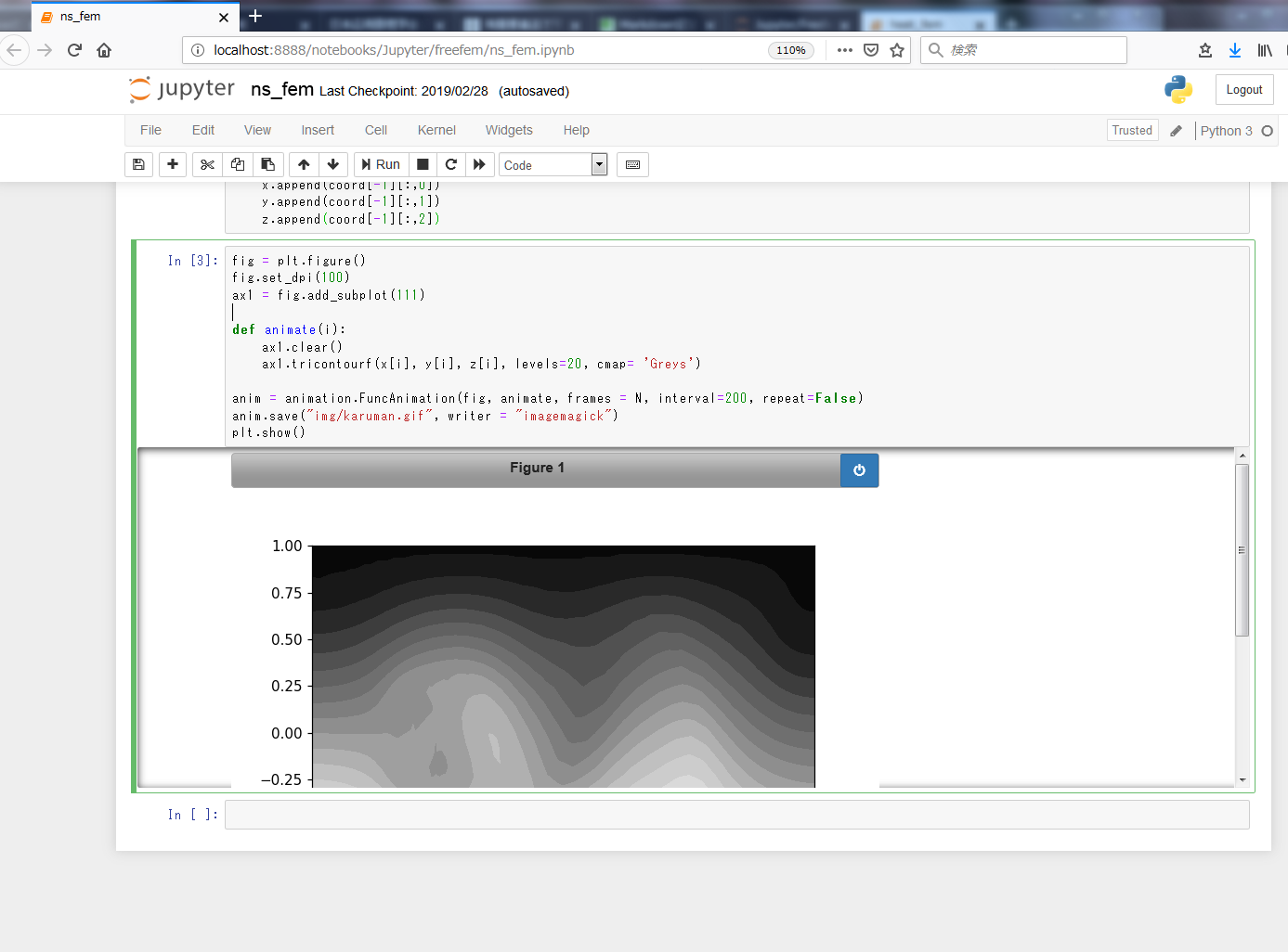
- 投稿日:2019-03-10T18:09:35+09:00
FreeFem++ と Python を使って数学 gif を作ってみよう
本記事では Windows を使っている人向けに、FreeFem++ という有限要素法を用いて偏微分方程式の数値計算を行うソフトウェアから計算結果を出力し、Python の matplotlib を用いて、物理的な時間発展現象を可視化する数学 gif を作ってみます。
いずれのソフトウェアも無料です。今回テーマとするのはカルマン渦列と熱拡散です。
左から流体が流れてきたとき、障害物の後方に渦の列が上下交互に現れているのがわかります。
熱が"冷めて"いく様子です。こんな感じの数学 gif を作っていきましょう!
1. FreeFEM++とmatplotlibをインストールしよう!
この章では@t_kemmochiさんのFreeFem++の紹介と以前の記事Python を使ってお手軽に数学 gif を作ってみようの前半部分を参考にお願いします。
1.1 FreeFEM++を手に入れよう!
@t_kemmochiさんのFreeFem++の紹介にしたがって、FreeFEM++の公式サイトからFreeFEM++をダウンロード&インストールした上で、専用の総合環境であるFreeFem++-csをダウンロードしましょう。
Macの人は上手く行かないことがあるようです。その場合は適当なエディダでコードを編集した後に、ターミナルから実行することでFreeFem++に計算させることになります。
1.2 matplotlib をインストールしよう!
未インストールの場合は Anaconda3 の導入から行ってください。例えば、
の前半部分を行えば大丈夫です(matplotlibのバージョンアップまで忘れずに行いましょう)
2 数値計算をして、計算結果を出力しよう!
数値計算のコードはプロが一般に公開しているものを流用させていただきます。
2.1 有限要素法によるカルマン渦列の数値計算をしよう!
大塚 厚二, 高石 武史. 「有限要素法で学ぶ現象と数理」のサポートサイトの第4章のサンプル(元は鈴木厚博士によるもの)をベースとしてカルマン渦列の数値計算をします。
matplotlib に読み込ませる csvファイルは@t_kemmochiさんのFreeFem++の紹介による方法を用います。
後での可視化の都合上、流れ関数 $\varphi$ はP1要素に変更しておきます(P2での出力・可視化の仕方は調査中です…)。
以下のようなコードに変更した後、ファイルを実行すると連番のcsvファイルが出力されます。
navier-stokes.edpmacro grad(u) [dx(u),dy(u)] // EOM macro div(u1,u2) (dx(u1)+dy(u2)) // EOM int i=0; real t=0; real nu = 1.0/400.0; real dt=0.1; // time step int imax=500; // max iteration steps int iplt0=imax/40; // interval for plot int iplt1=imax/10; // interval for ps file real alpha=1.0/dt; //境界条件 滑無,滑り,流入,流出 int wall=1, slide=2, inflow=4, outflow=5; border ba(t=0,1.0){x=t*5.0-1.0;y=-1.0;label=slide;}; // 下 border bb(t=0,1.0){x=4.0;y=2.0*t-1.0;label=outflow;}; // 右 border bc(t=0,1.0){x=4.0-5.0*t;y=1.0;label=slide;}; // 上 border bd(t=0,1.0){x=-1.0;y=1.0-2.0*t;label=inflow;}; // 左 border cc(t=0,2*pi){x=cos(t)*0.25;y=sin(t)*0.25;label=wall;}; mesh Th=buildmesh(ba(30)+bb(30)+bc(30)+bd(30)+cc(-30)); // P2/P1要素 fespace Vh(Th,[P2,P2]),Qh(Th,P1),Xh(Th,P1); Vh [u1,u2],[v1,v2],[up1,up2]; Qh p,q; Xh psi,phi,phii; problem NS([u1,u2,p], [v1,v2,q],solver=UMFPACK,init=i) = int2d(Th)( alpha*(u1*v1 + u2*v2) + nu*(grad(u1)'*grad(v1) + grad(u2)'*grad(v2)) - p*div(v1,v2) - q*div(u1,u2) ) - int2d(Th)( alpha*(convect([up1,up2],-dt,up1)*v1 + convect([up1,up2],-dt,up2)*v2) ) + on(slide,u2=0) // 壁境界 滑り + on(inflow,u1=1.0-y*y,u2=0) // 流入 $u_{1}=1-y^{2}$ + on(wall,u1=0,u2=0); // 壁境界 円柱 滑り無 phii = y-y*y*y/3.0; problem streamlines(phi,psi,solver=Crout,init=i) = // from cavity.edp int2d(Th)(dx(phi)*dx(psi)+dy(phi)*dy(psi)) - int2d(Th)((dx(u2)-dy(u1))*psi) + on(slide,phi=phii) + on(inflow,phi=phii) + on(wall,phi=0); [u1,u2] = [0,0]; // 初期条件 for ( i = 1; i <= imax; i++) { t=dt*i; [up1,up2]=[u1,u2]; // $\vec{u}^{n-1}$の更新 NS; // $\vec{u}^{n},p^{n}$の計算 streamlines; // 流線の計算 if (i%50 == 0) plot(phi,cmm="Streamlines t="+t,nbiso=40); if (i%5 == 0){ ofstream sol("csv/phi"+i/5+".csv"); for(int j=0;j<Th.nv;j++) sol << Th(j).x << "," << Th(j).y << "," << phi[][j] << endl; } }ここで、ファイルを保存する際にはedpファイルが置かれているフォルダにあらかじめ csv というフォルダを作っておきましょう。
2.2 有限要素法による熱方程式の数値計算をしよう!
こちらでは齊藤宣一教授の個人サイトからサンプルプログラムを探しましょう。
その中から、Heat.edp を見つけ出し、以下のように出力の形式を整えます。
Heat.edp/* Solving linear Heat equation du/dt - \Delta u = 0 in 2d ball B(0,R), u = 0 on boundary |x| = R, u(x,0) = 5*exp(5*(-x^2-y^2)); R = 1.0 */ real h = 0.02, R = 1; border C(t =0,2*pi){x=R*cos(t); y=R*sin(t);label=1;}; mesh Th = buildmesh(C(floor(2.*pi*R/h))); fespace Vh(Th,P1); real dt = 0.001, T = 0.2; Vh uh, vh, uh0 = 5*exp(5*(-x^2-y^2)); problem Heat(uh,vh) = int2d(Th)(uh*vh/dt) + int2d(Th)(dx(uh)*dx(vh) + dy(uh)*dy(vh)) - int2d(Th)(uh0*vh/dt) + on(1, uh=0); real t = 0; int k = 0; for(t = dt;t<T+dt/2;t+=dt){ cout<<"t="<<t; Heat; k++; if(k%2 == 0){ ofstream sol("csv/uh"+k/2+".csv"); for(int j=0;j<Th.nv;j++){ sol << Th(j).x << "," << Th(j).y << "," << uh[][j] << endl; } } uh0 = uh; } ofstream tri("csv/Th.csv"); for(int i=0;i<Th.nt;i++){ tri << Th[i][0] << "," << Th[i][1] << "," << Th[i][2] << endl; }こちらでも、ファイルを保存する際にはedpファイルが置かれているフォルダにあらかじめ csv というフォルダを作っておきましょう。
3 計算結果を jupyter に読み込ませて、数学 gif にしてみよう!
これで準備が整いました。jupyter notebook を起動して、次のようにしてライブラリの読み込み、csv の読み込み、グラフの出力を行います。
実行前に、作業中のフォルダにimgという名前のフォルダを作成しておきましょう。
ns_fem.ipynb%matplotlib nbagg import numpy as np import matplotlib.pyplot as plt import matplotlib.animation as animation import pandas as pd coord = [] x = [] y = [] z = [] N = 100 for i in range(N): coord.append(pd.read_csv('csv/phi'+str(i+1)+".csv",header=None).values) x.append(coord[-1][:,0]) y.append(coord[-1][:,1]) z.append(coord[-1][:,2]) fig = plt.figure() fig.set_dpi(100) ax1 = fig.add_subplot(111) def animate(i): ax1.clear() ax1.tricontourf(x[i], y[i], z[i], levels=20, cmap= 'Greys') anim = animation.FuncAnimation(fig, animate, frames = N, interval=200, repeat=False) anim.save("img/karuman.gif", writer = "imagemagick") plt.show()これでめでたくgifの出力と保存ができるようになりました
熱方程式についても、同様の方法でgifの作成をすることができます。
heat_fem.ipynb%matplotlib nbagg import numpy as np import matplotlib.pyplot as plt import matplotlib.animation as animation import matplotlib.tri as mtri from mpl_toolkits.mplot3d import Axes3D import pandas as pd coord = [] x = [] y = [] z = [] N = 100 for i in range(N): coord.append(pd.read_csv('csv/uh'+str(i+1)+".csv",header=None).values) x.append(coord[-1][:,0]) y.append(coord[-1][:,1]) z.append(coord[-1][:,2]) tridata = pd.read_csv('csv/Th.csv',header=None).values tri = mtri.Triangulation(x[0], y[0], triangles=tridata) fig = plt.figure() ax = fig.gca(projection='3d') def animate(i): ax.clear() ax.set_zlim(-0.,4.) ax.plot_trisurf(tri, z[i], cmap = plt.cm.jet, vmin = 0, vmax = 4) ax.set_xlabel('x') ax.set_ylabel('y') ax.set_zlabel('u') anim = animation.FuncAnimation(fig, animate, frames=N, interval=10, repeat = False) anim.save("img/heat_fem.gif", writer = "imagemagick") plt.show()
- 投稿日:2019-03-10T18:00:06+09:00
Jupyter NotebookでCTF(初級)
ハイレベルなCTFにはまったく歯が立たないが、いざというときに使えるようリストアップしてみた。
シーザー暗号
よく出てくるシーザー暗号。
def _rot13(c):
    if 'A' <= c and c <= 'Z':
        return chr((ord(c) - ord('A') + 13) % 26 + ord('A'))
    if 'a' <= c and c <= 'z':
        return chr((ord(c) - ord('a') + 13) % 26 + ord('a'))
    return c

def rot13(s):
    g = (_rot13(c) for c in s)
    return ''.join(g)
https://github.com/usop4/jupyter_sectools/blob/master/ksnctf_2_easy_cipher.ipynb
pycurl
curlをpythonから使えるようになると、パスワードリスト攻撃などを効率的にしやすくなる。(あ、もちろんCTFでの話ですよ・・・)
import pycurl
from io import BytesIO

buffer = BytesIO()
c = pycurl.Curl()
c.setopt(c.URL, 'http://ctfq.sweetduet.info:10080/~q32/auth.php')
c.setopt(c.WRITEDATA, buffer)
c.setopt(pycurl.POST, 1)
c.setopt(pycurl.HTTPPOST, [('password[1]', 'dummy'),('password[2]', 'dummy')])

c.perform()
c.close()

body = buffer.getvalue()
print(body.decode('iso-8859-1'))
https://github.com/usop4/jupyter_sectools/blob/master/ksnctf_12.ipynb
nc
import socket
import time

def mysend(s, message):
    time.sleep(0.1)
    message = message + '\n'
    s.send(message.encode())
    time.sleep(0.1)
    data = s.recv(1024).decode('utf-8').splitlines()[0]
    print(data)

s = socket.socket(socket.AF_INET, socket.SOCK_STREAM)
s.connect(('example.com', 1234))
numpy
numpyは多次元配列などを扱いやすくするモジュールだが、matplotlibと組み合わせて、計算結果をざっと確認するのに便利。
import numpy as np
import matplotlib.pyplot as plt

arr2d = []
arr2d.append([1,0])
arr2d.append([0,1])
arr2dnp = np.asarray(arr2d)
plt.imshow(arr2dnp)
バイナリ、文字列
print(chr(int('0b01110100',0))) # tcrypt
最後にcrypt。ksnctfのJohnという問題はJohn the ripperというプログラムを使ってパスワードリストから総当たりするのが王道かもしれないが、Pythonのcryptで解くのもスマートな感じで気持ち良い。
https://ksnctf.sweetduet.info/problem/14
import crypt

s = '''
user00:$6$Z4xEy/1KTCW.rz$Yxkc8XkscDusGWKan621H4eaPRjHc1bkXDjyFtcTtgxzlxvuPiE1rnqdQVO1lYgNOzg72FU95RQut93JF6Deo/:15491:0:99999:7:::
user01:$6$ffl1bXDBqKUiD$PoXP69PaxTTX.cgzYS6Tlj7UBvstr6JruGctoObFXCr4cYXjIbxBSMiQZiVkKvUxXUC23zP8PUyXjq6qEq63u1:15491:0:99999:7:::
user02:$6$ZsJXadT/rv$T/2gVzYwMBaAsZnHIjnUSmTozIF/ebMvtHIJjikFehvB8pvy28DUIQYbTJLG6QAxhzJAKOROnZq0xV4hUGefM1:15491:0:99999:7:::
'''

salt = []
hash = []
for line in s.splitlines():
    m = line.split(":")
    n = m[1].split("$")
    hash.append(m[1])
    salt.append(n[2])

password = []
for line in open('password_list.txt', 'r'):
    password.append(line.strip())

for s in salt:
    for p in password:
        h = crypt.crypt(p, salt='$6$'+s+'$')
        if h in hash:
            print(p)
            break
- 投稿日:2019-03-10T17:39:22+09:00
【ひらけごま】STFT,VGG16-like,そしてPyaudioで「エッジ音声認識アプリ」を作ってみた♬垂れ流し改善編
昨夜のアプリ、どんどん垂れ流しアプリなので、今後の利用のために少し改善して待てるようにしました。
つまり、ファイルの格納ディレクトリから一度だけ読み込むように、
①ファイルの存在チェックを実施
②読込んだらファイル消去
というのを追加して、新規に声を取得したら反応するように改善しました。
合わせて流れを変更して読込初期の揺らぎを改善しました。やったこと
・ファイル存在チェックの追加
・読み込んだらファイル消去
・コード解説・ファイル存在チェックの追加
【参考】
・pythonでファイルの存在を確認する
参考のとおりに以下で実施できます。import os path = "./out_test/figure.jpg" os.path.exists(path)これで./out_test/にfigure.jpgが存在するかどうかの判定ができます。
Trueで存在、Falseで存在しない。
ということで、存在を確認してから読み込むというシーケンスが作成できます。・読み込んだらファイル消去
上記と対の機能がファイルを読み込んだら、二度目は読み込まないように消去しておきたいところです。
ということで、以下の参考が役に立ちます。
【参考】
・ファイルやフォルダーを削除する
つまり、参考のとおり、以下で実施できました。import os path = "./out_test/figure.jpg" os.remove(path)ちなみに、参考ではディレクトリの削除やディレクトリツリーごと削除も掲載されています。
・コード解説
上記二つの機能を盛り込んで以下のように変更しました。
学習などは変わらないので昨夜の記事を見てください。
import osを追記しています。
昨夜のコード
hirakegoma / out_onsei.py
hirakegoma / pyaudio_realtime_last.pyout_onsei_improve.py#-*- cording: utf-8 -*- import numpy as np #np.random.seed(1337) # for reproducibility import wave import pyaudio from vgg16_like import model_family_cnn from keras.preprocessing import image import matplotlib.pyplot as plt import keras from keras.preprocessing import image import ospredictionに変更はありません。
out_onsei_improve.pydef prediction(imgSrc): img = np.array(imgSrc) img = img.reshape(1, img_rows,img_cols,3) img = img.astype('float32') img /= 255 t0=time.time() y_pred = model.predict(img) return y_predwhile前に
path = "./out_test/figure.jpg"
を定義しました。out_onsei_improve.pynum_classes = 2 img_rows,img_cols=128, 128 input_shape = (img_rows,img_cols,3) #224, 224, 3) model = model_family_cnn(input_shape, num_classes = num_classes) # load the weights from the last epoch model.load_weights('params_hirakegoma-61.hdf5', by_name=True) print('Model loaded.') path = "./out_test/figure.jpg"while True:の中で最初に
if os.path.exists(path)==True:
として、存在すれば以下を実行するように変更しました。
また、音声を新たに入力してpathに格納するとき、タイミングを計るために
for i in range(100000): i += 1
を入れました。
また、最後のところでファイルの削除を実施しています。if input==b'': os.remove(path) breakそれ以外は変更していません。
out_onsei_improve.pywhile True: imgSrc=[] if os.path.exists(path)==True: for i in range(100000): i += 1 imgSrc = image.load_img("./out_test/figure.jpg", target_size=(img_rows,img_cols)) plt.imshow(imgSrc) plt.pause(1) plt.close() pred = prediction(imgSrc) print(pred[0]) if pred[0][0]>=0.5: filename = "ohayo.wav" print("ohayo") else: filename = "hirakegoma.wav" print("hirakegoma") # チャンク数を指定 CHUNK = 1024 #filename = "hirakegoma.wav" wf = wave.open(filename, "rb") # PyAudioのインスタンスを生成 p = pyaudio.PyAudio() # Streamを生成 stream = p.open(format=p.get_format_from_width(wf.getsampwidth()), channels=wf.getnchannels(), rate=wf.getframerate(), output=True) # データを1度に1024個読み取る input = wf.readframes(CHUNK) # 実行 while stream.is_active(): output = stream.write(input) input = wf.readframes(CHUNK) #print(input) if input==b'': os.remove(path) break # ファイルが終わったら終了処理 stream.stop_stream() stream.close() p.terminate()また、音声録音側のアプリは以下のように変更しました。
実は、前回のコードだと測定開始時にミスって、変なデータを格納してから正しいデータを格納していました。
そこで、start_measure():の変数にp1のように1をつけました。
※これ最終的には不要でした
ということで、基本的に最初の部分は変更なしです。pyaudio_realtime.py# -*- coding:utf-8 -*- import pyaudio import time import matplotlib.pyplot as plt import numpy as np import wave from scipy.fftpack import fft, ifft from scipy import signal import os def start_measure(): CHUNK=1024 RATE=44100 #11025 #22050 #44100 p1=pyaudio.PyAudio() input1 = [] stream1=p1.open(format = pyaudio.paInt16, channels = 1, rate = RATE, frames_per_buffer = CHUNK, input = True) input1 =stream1.read(CHUNK) sig1 = np.frombuffer(input1, dtype="int16")/32768.0 while True: if max(sig1) > 0.001: break input1 =stream1.read(CHUNK) sig1 = np.frombuffer(input1, dtype="int16")/32768.0 stream1.stop_stream() stream1.close() p1.terminate() return以下のコードも基本はあまり変更なく、
以下の設定を毎回初期化するようにfor s in range(0,900,1):
の中に入れました。これで最初に変な録音が入るバグが解消しました。
※昨夜のバージョンだと垂れ流しで変な録音が入ってもファイル取得前に上書きされてノイズが見えていませんでしたが、今回は一個一個取得ー消去をするのでより鮮明になってバグが発見できましたstream=p.open(format = pyaudio.paInt16, channels = 1, rate = RATE, frames_per_buffer = CHUNK, input = True)したがって、以下のパラメータ部分のみ外だししています。
pyaudio_realtime.pyfig = plt.figure(figsize=(6, 5)) ax2 = fig.add_subplot(111) N=50 CHUNK=1024*N RATE=44100 #11025 #22050 #44100 p=pyaudio.PyAudio() fr = RATE fn=51200*N/50 fs=fn/fr for s in range(0,900,1): print(s) start_measure() stream=p.open(format = pyaudio.paInt16, channels = 1, rate = RATE, frames_per_buffer = CHUNK, input = True) input = [] start_time=time.time() input = stream.read(CHUNK) stop_time=time.time() sig =[] sig = np.frombuffer(input, dtype="int16") /32768.0 nperseg = 1024 f, t, Zxx = signal.stft(sig, fs=fn, nperseg=nperseg) ax2.pcolormesh(fs*t, f/fs/2, np.abs(Zxx), cmap='hsv') ax2.set_xlim(0,fs) ax2.set_ylim(20,20000) ax2.set_yscale('log') ax2.set_axis_off() plt.pause(0.01) plt.savefig('out_test/figure.jpg') #output = stream.write(input) stream.stop_stream() stream.close() p.terminate() print( "Stop Streaming")結果
こうして以下のとおり、録音と読込の記録の数が一致するようになりました。
>python pyaudio_realtime.py
0
1
2
3
4
5
6
7
8
ちょっと1より小さい数字が出ているところは「おはー」とか録音している部分です。
※0は録音前に表示されているので、以下の方が一個少ないですModel loaded. 2019-03-10 17:07:16.052326: W ... [ 2.01997850e-07 9.99999762e-01] hirakegoma [ 1.00000000e+00 8.13874673e-33] ohayo [ 0.00337285 0.99662721] hirakegoma [ 1.00000000e+00 1.21284272e-29] ohayo [ 1.00000000e+00 1.55338318e-34] ohayo [ 1.00000000e+00 6.55481190e-15] ohayo [ 4.60651776e-25 1.00000000e+00] hirakegoma [ 1.00000000e+00 1.52230811e-10] ohayo forrtl: error (200): program aborting due to control-C eventまとめ
・録音データ(スペクトログラム)の保存ー消去を実施したので、余裕をもって一つずつ処理ができるようになった
・読み込むデータの時間軸の初期値が安定した・少し長めの文章に挑戦したいと思う
- 投稿日:2019-03-10T17:06:17+09:00
【データサイエンス】データサイエンスによく使われるscikit-learnを学ぶ
はじめに
こんにちは、皆さん!@Raphael_de_murlです。今回は機械学習やデータサイエンスの処理でよく使われるライブラリをご紹介したいと思います。
scikit-learnとは
以下はscikit-learn - Wikipediaの定義です。scikit-learn (旧称:scikits.learn) はPythonのオープンソース機械学習ライブラリである。サポートベクターマシン、ランダムフォレスト、Gradient Boosting、k近傍法、DBSCANなどを含む様々な分類、回帰、クラスタリングアルゴリズムを備えており、Pythonの数値計算ライブラリのNumPyとSciPyとやり取りするよう設計されている。
結構目に慣れたライブラリ名が見えてますね。説明の通りscikit-learnはSVMとかRandom Forestとかk近傍法とか色んな機械学習関連のライブラリとよく使われてますので基本からしっかり身につける必要がありますと思ってます。
scikit-learnの特徴
scikit-learn アルゴリズム・チートシート
上記のの画像はscikit-learnのアルゴリズムチートシートです。多分機械学習を勉強している方や現役で使っている方はよく見た画像だと思います。これらは機械学習を行う際、やりたい処理に対しどのモデルを選んでやるのかをscikit-learnがサポートしてくれるっていう風に理解すれば大丈夫だと思います。この4つの分析を軽く見てみます。classification(分類)は2つ以上の離散カテゴリへの分類ラベルを予測するモデルとしてクラス分類問題や教師あり学習で使われます。
- SGD classifier
- 大規模のデータの線形のクラス分類手法です。
- Linear SVC
- SGDよりは小さな中小規模のデータの線形のクラス分類手法です。
- KNeighbors Classifier
- こちらはLinear SVCでうまく分類ができてなかった場合に利用する非線形クラス分類手法で中小規模のデータを扱います。
- kernel approximation
- こちらはSGDでうまく分類ができてなかった場合に利用する非線形クラス分類手法で中小規模のデータを扱います。
regression(回帰)は連続ラベルを予測するモデルとして教師あり学習で使われます。
- SGD regressor
- 大規模のデータの線形の回帰分析の手法です。
- Lasso、ElasticNet
- 中小規模で説明変数の一部が重要な場合に使われる、回帰分析の手法です。
- RidgeRegression、SVR(kernel=linear)
- 中小規模で説明変数の全てが重要な場合に使われる、回帰分析の手法です。
- SVR(kernel)、EnsembleRegression
- こちらはRidge回帰やSVR(linear)で分析がうまくできなかった場合に利用する非線形の分析手法です。
clustering(クラスタリング)はデータ内のグループを検出して識別するモデルとしてラベルなしデータのラベルを推定する教師なし学習で使われます。
- KMeans
- いくつのクラスタに分かれるのか、事前に決めることができる場合におすすめな、クラスタリング分析手法です。
- Special Clustering、GMM
- KMeansでうまくクラスタリングが出来なかった場合に利用する非線形の分析手法です。
- Meanshift、VBGMM
- こちらはKMeansとは逆でクラスタに分かれるのか、決める事が出来ない場合に利用するクラスタリンくの分析手法です。
- MiniBatch KMeans
- こちらはデータが大規模の場合に使われるKMeansとしてデータを分けながら学習させる手法です。
dimentionality reduction(次元削減)はより高次元データ内の低次元構造を検出し識別するモデルとしてラベルなしデータの構造を推定する教師なし学習で使われます。
- Randomized PCA
- 多次元のデータから「意味のある特徴量」を特定したり、新たな軸を作る(基底を変換する)ことで、少ない変数でデータを再現します。
- Isomap, Spectral Embedding
- PCAが機能しない非線形な構造を持つデータにおいて、データ数が膨大でない場合に使用されます。
- LLE
- 非線形な構造を持つデータにおいて、Isomapがうまくいかない場合に、LLEが使用されます。
- kernel appoximation
- カーネルトリックを用いて、データを非線形変換した後にPCAを実施する方法です。
まとめに
説明が綺麗ではないんですけれども如何でしたでしょうか?いつも思うんですが大きな目的は皆さんと情報を共有したい!という気持ちでやっていますがまずが自分が勉強するための記事でもありますのでこれをご理解頂ければと思っております。次回は実際scikit-learnを用いた簡単な例をやって行きたいと思います。この記事が少しでも気に入った方はいいねとツイッターのフォロワー宜しくお願い致します。
レファレンス

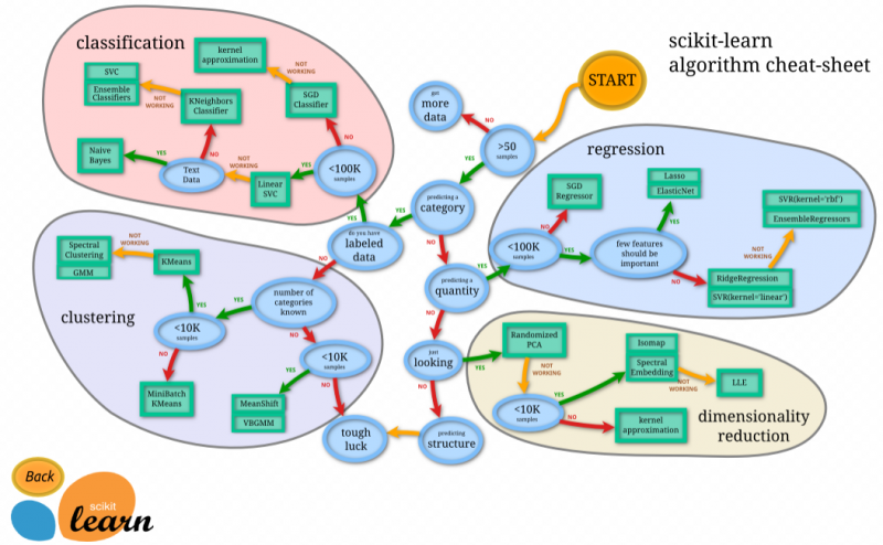
- 投稿日:2019-03-10T15:58:01+09:00
JWSANデータセットで単語ベクトルの性能評価 [memo]
JWSAN1 とは、日本語単語類似度・関連度データセットです。ここでは、単語ベクトルの評価にこのデータセットを使ってみます。
事前準備
- https://github.com/sugiyamath/jawiki2w2v を使ってword2vecモデルをjawikiから生成します。(おすすめは、t82w.pyを編集して、sg=0, sg=1の2つのパラメータのモデルを作成し比較することです。)
wget http://www.utm.inf.uec.ac.jp/JWSAN/jwsan-1400.csvします。評価コード
from gensim.models.word2vec import Word2Vec
import pandas as pd
import numpy as np


def load(modelpath, datapath):
    model = Word2Vec.load(modelpath)
    df = pd.read_csv(datapath)
    return model, df


def cossim(x,y):
    return np.dot(x,y)/(np.linalg.norm(x)*np.linalg.norm(y))


def eval_model(model, df, dim=200):
    out = {}
    diffs = []
    for i,d in df.iterrows():
        z = d['similarity']/6.0
        try:
            x = model.wv[d['word1']]
            y = model.wv[d['word2']]
            w = cossim(x,y)
        except Exception as e:
            w = 0.0
        out[d['pairID']] = {'true':float(z), 'pred':float(w)}
        diffs.append((z-w)**2)

    result = {"data":out, "global_score":float(np.mean(diffs))}
    return result


if __name__ == "__main__":
    import json
    modelpath = "./mymodel.model"
    datapath = "./jwsan-1400.csv"
    model, df = load(modelpath, datapath)
    result = eval_model(model, df)
    with open("result.json", "w") as f:
        json.dump(result, f)
注意
0〜6の評価値が与えられる、とデータセットの説明が書かれているため、それを6で割った値で類似度として比較していますが、この比較に合理的な理由があるかは不明です。cossimで与えられた類似度(予測値)と人間の手で与えた類似度(正解値)が比較可能なのかは注意する必要があります。
- 投稿日:2019-03-10T15:03:03+09:00
Python: アフィン変換
アフィン変換
opencvにアフィン変換はあるが, ちょいと遊びで自作してみた.
今回は画像を読み込んで, 回転しても範囲外に出ないように縁を付けた後変換するような処理で実装した.affin.pyimport cv2 import numpy as np from IPython.display import display, Image def display_cv_image(image, format='.png'): decoded_bytes = cv2.imencode(format, image)[1].tobytes() display(Image(data=decoded_bytes)) def add_edge(img): H, W = img.shape WID = int(np.max(img.shape) * 2**0.5) e_img = np.zeros((WID, WID)) e_img[int((WID-H)/2):int((WID+H)/2), int((WID-W)/2):int((WID+W)/2)] = img return e_img def affin(img, a, tx=0, ty=0): e_img = add_edge(img) WID = np.max(e_img.shape) x = np.tile(np.linspace(-1, 1, WID).reshape(1, -1), (WID, 1)) y = np.tile(np.linspace(-1, 1, WID).reshape(-1, 1), (1, WID)) p = np.array([[x, y, np.ones(x.shape)]]) t = np.array([[np.cos(a), -np.sin(a), -tx], [np.sin(a), np.cos(a), -ty], [ 0, 0, 1]]) dx, dy, _ = np.sum(p * t.reshape(*t.shape, 1, 1), axis=1) u = np.clip((dx + 1) * WID / 2, 0, WID-1).astype('i') v = np.clip((dy + 1) * WID / 2, 0, WID-1).astype('i') return e_img[v, u]今回はJupyter上でOpenCVを用いて画像表示を行うために以下を参考にdisplay_cv_imageを用意した.
http://uphy.hatenablog.com/entry/2016/12/11/110703def display_cv_image(image, format='.png'): decoded_bytes = cv2.imencode(format, image)[1].tobytes() display(Image(data=decoded_bytes))回転させても範囲外に出ないように縁をつける処理はこんな感じ.
まぁアフィン変換の本質の部分じゃないので( ´_ゝ`)フーンってみてもらえれば・・・
(ただ,縁をつけると正方形になるようになっていることはそこそこ大事かも?)def add_edge(img): H, W = img.shape WID = int(np.max(img.shape) * 2**0.5) e_img = np.zeros((WID, WID)) e_img[int((WID-H)/2):int((WID+H)/2), int((WID-W)/2):int((WID+W)/2)] = img return e_imgこれが実装したアフィン変換
def affin(img, a, tx=0, ty=0):
    e_img = add_edge(img)
    WID = np.max(e_img.shape)
    x = np.tile(np.linspace(-1, 1, WID).reshape(1, -1), (WID, 1))
    y = np.tile(np.linspace(-1, 1, WID).reshape(-1, 1), (1, WID))
    p = np.array([[x, y, np.ones(x.shape)]])
    t = np.array([[np.cos(a), -np.sin(a), -tx],
                  [np.sin(a),  np.cos(a), -ty],
                  [        0,          0, 1]])
    dx, dy, _ = np.sum(p * t.reshape(*t.shape, 1, 1), axis=1)
    u = np.clip((dx + 1) * WID / 2, 0, WID-1).astype('i')
    v = np.clip((dy + 1) * WID / 2, 0, WID-1).astype('i')
    return e_img[v, u]
まず縁をつけて幅x高=WIDxWIDの画像にする.
    e_img = add_edge(img)
    WID = np.max(e_img.shape)
次に上端から下端まで-1から1に変化するxと左端から右端まで-1から1に変化するyをもつ点のpをWIDxWIDのマップとして作る.
この時pの構造は3×WID×WIDx = np.tile(np.linspace(-1, 1, WID).reshape(1, -1), (WID, 1)) y = np.tile(np.linspace(-1, 1, WID).reshape(-1, 1), (1, WID)) p = np.array([[x, y, np.ones(x.shape)]])あとはこの各点をアフィン変換で目的の座標に変換する. 簡単化のため今回は引数で回転と並行移動のみあたえる.
(引数でこのtを渡す形式にすれば他の変換もできるようになる)t = np.array([[np.cos(a), -np.sin(a), -tx], [np.sin(a), np.cos(a), -ty], [ 0, 0, 1]]) dx, dy, _ = np.sum(p * t.reshape(*t.shape, 1, 1), axis=1)変換後のdx, dyは画像の座標系ではないので画像の座標系に変換して元画像の対応する点を取ってくると完成!
    u = np.clip((dx + 1) * WID / 2, 0, WID-1).astype('i')
    v = np.clip((dy + 1) * WID / 2, 0, WID-1).astype('i')
    return e_img[v, u]
テスト
テストに用いる画像を読み込む. 今回はlenaさんを用いた.
img = cv2.imread('lena.jpg', 0)
display_cv_image(img, '.png')
エッジをつける処理はこんな感じ
display_cv_image(add_edge(img), '.png')
アフィン変換で45度回転
display_cv_image(affin(img, np.pi/4), '.png')
平行移動も一応実装. 第3引数でx方向, 第4引数でy方向に移動させることができる.
(今回は1.0が画像半分の長さ相当)display_cv_image(affin(img, 0, 1.0), '.png')
まとめ
とりあえず回転と平行移動を簡単に行うaffin変換を実装した.
また, tを変えると拡大縮小や画像をゆがませることもできる(確認済)追記
今回作ったアフィン変換はラドン変換という別の変換行うために特化した仕様なので使い勝手は良くないかも・・・


- 投稿日:2019-03-10T12:41:55+09:00
TensorboardのEmbeddingによる高次元データの可視化
Tensorboard: Embedding
TensorbordのEmbeddingを利用することで高次元データを2/3次元での可視化が可能です。
公式ドキュメント等詳しく書かれていますが、備忘録を兼ねてコードを紹介したいと思います。TensorFlow Embedding: https://www.tensorflow.org/guide/embedding
Embedding デモ: https://projector.tensorflow.org/次元削減
次元の圧縮方法としては
PCAまたはt-SNEが利用可能ですす。Tensorboard実行時にはPCAによる削減がデフォルトで行われます。
注意点として、t-SNEによる次元削減では入力が50次元を超える場合、50次元まで落とした後にt-SNEによる削減を行っている(githubのissueで見かけたがリンクを忘れてしまった)。このため、sklearn等によるt-SNEの結果と一致しないようです。Python用コード
手順としては
1. projectorの設定ファイルを書き出す
2. checkpointファイルを書き出す
これだけです。環境
- Python: 3.6
- tensorflow: 1.10.0
- pandas: 0.24.1
コード
embedding.pyimport tensorflow as tf from tensorflow.contrib.tensorboard.plugins import projector from pathlib import Path import pandas as pd def embedding(vectors, save_dir, labels=None): with tf.Session() as sess: save_dir = Path(save_dir) if not save_dir.exists(): save_dir.mkdir(parents=True) vectors_tensor = tf.Variable(vectors) sess.run(tf.global_variables_initializer()) save = tf.train.Saver() save.save(sess, save_dir.joinpath('embedding.ckpt').as_posix()) config = projector.ProjectorConfig() embedding = config.embeddings.add() embedding.tensor_name = vectors_tensor.name if labels is not None: embedding.metadata_path = 'label.tsv' label_df = pd.DataFrame({'Label': labels}) label_df.to_csv(save_dir.joinpath('label.tsv'), sep='\t', index=False, header=False) summary_writer = tf.summary.FileWriter(save_dir.as_posix()) projector.visualize_embeddings(summary_writer, config)可視化したいサイズ
(データ数, 次元数)のベクトルデータと保存先を与えることで指定ディレクトリにcheckpointファイルを書き出してくれる。データ数に一致するラベルを与えることでデータにラベルを付加することも可能です。
なお、10,000点を超えるデータは実行時に10,000点がランダムに選択されて可視化されます。実行
実行はいつも通り
tensorboardを実行後、ブラウザでアクセスするだけです。$ tensorboard --logdir path/to/logdir

- 投稿日:2019-03-10T11:53:25+09:00
Django Rest Framework で親子関係のあるテーブルにデータを登録する
はじめに
1つのエンドポイントで、親子関係があるテーブル構造に対してどうやってデータを登録するんだろうか。
業務中にそんな事があったので、記載します。目次
1. 要件
2. リクエストAPIのデータ構造
3. モデルの定義
4. Viewの定義
5. Serializerの定義
6. URLディスパッチャの定義
7. 動作の確認
8. まとめ1. 要件
今回は、「受注をする」という要件を想定して作業をしてみようと思います。
ECなどでよくある受注機能ですね。
受注ヘッダ(orderhead)、受注明細(orderdetail)という1対多の
親子関係を持ったテーブル構造に対してデータを登録することをゴールにします。2. リクエストAPIのデータ構造
まずDjango側で受けるPOSTデータの定義をしようと思います。
以下のように、受注ヘッダの基となるデータ群(親)と、受注明細の基となるデータ群(子)を
定義しました。order.json{ "order_number" : "9000000", "customer_id" : "customer001", "order_detail": [ { "product_code":"A001", "quantity":2 }, { "product_code":"A002", "quantity":2 } ] }3. モデルの定義
データを格納するテーブル構造を以下に記載します。
受注ヘッダ(OrderHead)と受注明細(OrderDetail)です。
受注明細側には、Foreignキーを利用して受注ヘッダと受注明細に1対多の関係を築きます。models.pyclass OrderHead(models.Model): order_number = models.CharField(max_length=10) order_at = models.DateTimeField(auto_now_add = True) customer_id = models.CharField(max_length=12) class OrderDetail(models.Model): orderhead = models.ForeignKey(OrderHead, related_name='details', on_delete=models.CASCADE) product_code = models.CharField(max_length=10) quantity = models.PositiveSmallIntegerField()4. Viewの定義
リクエストデータを受けたあとに、どう処理するかを記述します。
極力Django Rest frameworkの機能を活かそうとModelViewSetsを利用してます。view.pyclass OrderViewSet(viewsets.ModelViewSet): queryset = OrderHead.objects.all() serializer_class = OrderSerializer def create(self, request): order_serializer = OrderSerializer(data=request.data) if not order_serializer.is_valid(): print(order_serializer.errors) return Response("validation error........") result = order_serializer.save() return Response(result)5. Serializerの定義
view側からの呼び出しで、リクエストデータに対しての処理を記述します。
ModelSerializerを利用することでリクエストデータと、モデルフィールドのマッピングをして
バリデーションチェックやデータ登録処理を行うようにします。
※バリデーションは、modelフィールドに基づいて実施order_haed、order_detailへデータ登録した際のサロゲートキー(自動採番キー)を取得して
レスポンスデータとして返却する仕組みにしました。serializer.pyclass OrderDetailSerializer(serializers.ModelSerializer): class Meta: model = OrderDetail fields = ('product_code','quantity') class OrderSerializer(serializers.ModelSerializer): order_detail = OrderDetailSerializer(many=True) class Meta: model = OrderHead fields = ('order_number','customer_id', 'order_detail') def create(self, validated_data): result_dict = {} detail_list = [] order_detail = validated_data.pop('order_detail') created_orderhead = OrderHead.objects.create(**validated_data) result_dict['head_id'] = created_orderhead.id for order_detail_data in order_detail: created_orderdetail = OrderDetail.objects.create(orderhead=created_orderhead, **order_detail_data) detail_list.append(created_orderdetail.id) result_dict['detail_id'] = detail_list return result_dict6. URLディスパッチャの定義(URLConf)
アプリケーション毎のurls.pyの設定は以下になります。
受注の操作を可能とするAPIなので、ordersを定義して、このURLに対して
HTTPメソッドを指定することで、動作を行うようにします。urls.py# coding: utf-8 from rest_framework import routers from .views import OrderViewSet router = routers.DefaultRouter() router.register(r'orders', OrderViewSet)7. 動作の確認
Postmanを利用して確認します。
レスポンスが返ってきていることが分かります。
続いてDBに登録されているか確認します。
oderheadテーブルのidがレスポンスで返ってきた値と一緒であることが分かります。・orderheadテーブル確認
・orderdetailテーブル確認
8. まとめ
受注ヘッダと受注明細にデータを登録するAPIを作成することができました。
作成して思ったことは、serializerは、OrderSerializerが1つあって、その中でOrderHeader,OrderDetailのserializerを読む形ができればもっと綺麗な形で
デザインできたんじゃないかと思います。
今日はここまで。
最後まで読んでくださった方 ありがとうございました。
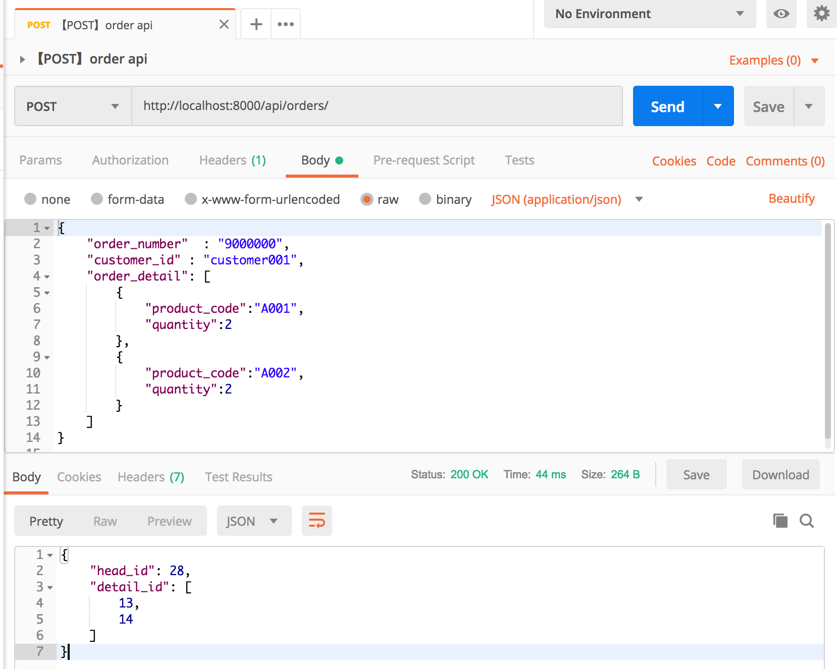
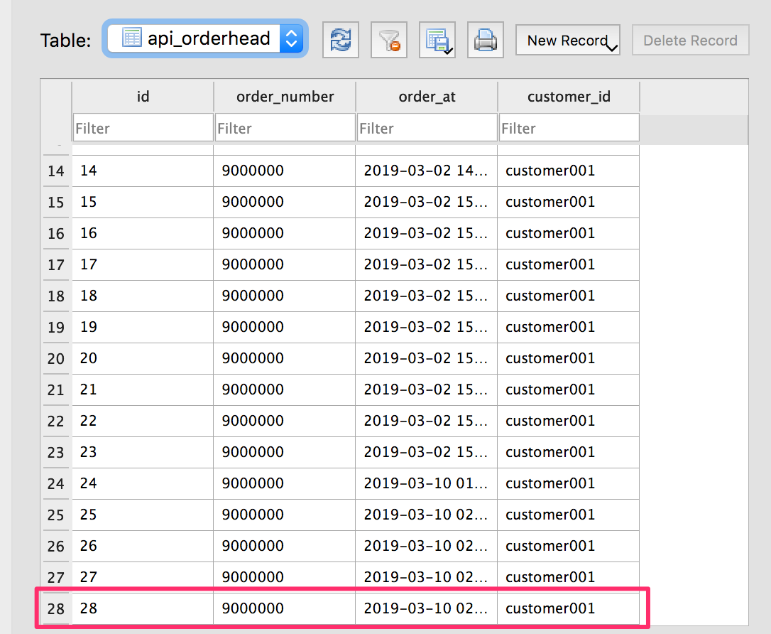
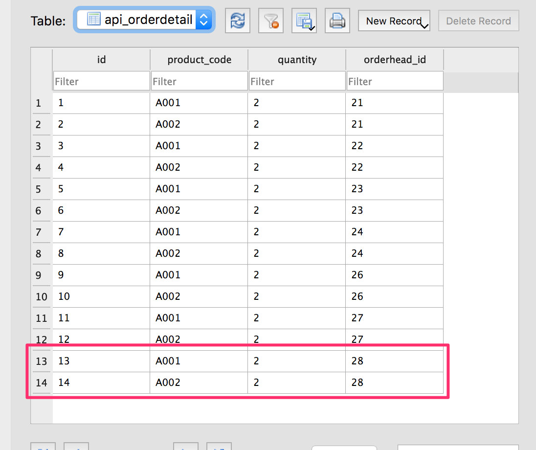
- 投稿日:2019-03-10T11:40:11+09:00
AWS StepFunctions を使った機械学習ワークフローの管理
本記事でやること
AWS StepFunctionsを使って、トレーニングからエンドポイントの作成までの以下ワークフローを作成する。
- 1.S3にトレーニング用のデータファイルが存在しているのかのチェック
- 2.SageMakerによるトレーニングジョブの開始
- 3.トレーニングジョブが開始された事をSlackに通知
- 4.トレーニングが終了するまでステータスを監視してポーリング
- 5.トレーニングが終了した事をSlackに通知
- 6.学習モデルのデプロイ、エンドポイントの作成(または更新)
- 7.エンドポイントが作成されるまでステータスを監視してポーリング
- 8.エンドポイントが作成(または更新)された事をSlackに通知
上記のワークフローをCloudFormationを使って作成する。
AWS公式が公開しているワークフローを参考にして作成をしております。
(トレーニングデータを置いているS3のPrefixなど想定しているケースが異なる箇所があるので所々改変して作成しております)本記事でやらないことは以下の通りなので、私が以前書いた記事を参照してください。
- トレーニングジョブ用のDocker imageのAWS ECRへのPush(こちらを参照してください)
- 各種IAMの設定
また、今回書いたコードはGithubに上げておりますので、適宜ご参照して頂ければと思います。
対象読者
- AWS SageMakerを使ってトレーニングや推論までを行なった事がある方
- AWS StepFunctionsに関して一通りの知識がある方
使用言語
- Python 3.6.3
想定ケース
- トレーニングを行う対象のデータは、前日に作成されたファイルを使用する
- S3のPrefix及びデータファイル名は以下の構成
input-data-trainingなどのフォルダ以下に日付のフォルダを作成する。- トレーニングを行う日付は、StepFunctions実行時に環境変数として与える。
bucket
  ├── input-data-training
  │    └── YYYY-MM-DD
  │          └── multiclass
  │               └── iris.csv # 対象のデータファイル
  │
  ├── input-data-validation
  │    └── YYYY-MM-DD
  │          └── multiclass
  │               └── iris.csv # 対象のデータファイル
  ├── input-data-prediction
  │    └── YYYY-MM-DD
  │          └── multiclass
  │               └── iris.csv # 対象のデータファイル
  └── output-model
       └── YYYY-MM-DD
             └── multiclass
                  └── training-job-name
                       └── output
                             └── model.tar.gz # 学習モデル
使用するファイル及びフォルダの構成
StepFunctionsをCloudformationで作成する際に使用するファイルと構成は以下の様になります。
最初にlambda_scriptsの説明を行い。その後に、Stepfunctionsの定義ファイルやCloudformationのテンプレートファイルの説明を行います。. ├── cloudformation │ ├── cloudformation.yml # cloudformation定義用ファイル │ └── cloudformation.yml.tpl # cloudformation定義用ファイルのテンプレート │ ├── create-stack.sh # cloudformationのスタック作成ファイル ├── delete-stack.sh # cloudformationのスタック削除ファイル │ ├── formation_config_creator.py # cloudformationテンプレートファイルにレンダリングするファイル │ ├── lambda_scripts │ ├── data_checker.py # トレーニング用データファイルの存在を確認 │ ├── deploy_model.py # 学習モデルのデプロイ~エンドポイントの作成 │ ├── get_status.py # SageMaker上でのトレーニングジョブ・エンドポイント作成のステータスを取得 │ ├── notify_slack.py # slack通知 │ └── start_training_job.py # トレーニングジョブの開始 │ └── stepfunctions └── state_machine.json # StepFunctionsの定義今回作成するワークフローの説明
トレーニング時のワークフロー概要
1. S3の該当バケットに前日分のトレーニングデータが存在しているのかチェック
以下のファイルで行なっている内容は、
- StepFunctions実行時に与えられた日付の前日の日付を取得
- S3の対象Prefixに指定したファイル名が存在しているのかをチェック
- 存在していれば、
日付とS3のinput-data-path、output-data-pathvalidation-data-pathendpointに値を入れ返す。またno_new_dataにfalseを入れる。- 存在していなければ、
no_new_dataにtrueを入れて返す。data_checker.pyimport os import logging import boto3 from datetime import datetime, timedelta, timezone # データ確認用のバケット BUCKET = "sample-bucket" # 存在を確認するファイル名 FILE_NAME = "iris.csv" # エンドポイント名 ENDPOINT_NAME = "multiclass" # loggerの作成 LOGGER = logging.getLogger() LOGGER.setLevel(logging.INFO) def lambda_handler(event, _context): LOGGER.info(event) s3_client = boto3.client("s3") # 指定された日付の前日の日付を取得 one_days_before = add_days(event["DATE"], -1) # 前日分の訓練データが存在するのか確認 status = check_data(s3_client, one_days_before) if status is not True: print('No new data uploaded since last training run.') print('Skipping training until next scheduled training run.') return { "no_new_data": True } s3_input_path, s3_output_path, s3_valid_path = generate_s3_path(one_days_before) return { "time": one_days_before, "s3_input_path": s3_input_path, "s3_output_path": s3_output_path, "s3_valid_path": s3_valid_path, "no_new_data": False, "endpoint": ENDPOINT_NAME } def check_data(s3_client, date): prefix = "input-data-training" response = s3_client.list_objects( Bucket=BUCKET, Prefix=prefix ) assumed_keys = [f'input-data-training/{date}/multiclass/{FILE_NAME}'] try: keys = [content['Key'] for content in response['Contents']] print("keys:", keys) status = set(assumed_keys).issubset(keys) except KeyError: status = False return status def generate_s3_path(date): train_set_prefix = os.path.join('input-data-training', date, 'multiclass') output_set_prefix = os.path.join("output-model", date, "multiclass") validation_set_prefix = os.path.join("input-data-validation", date, "multiclass") s3_input_path = os.path.join('s3://', BUCKET, train_set_prefix, '') s3_output_path = os.path.join('s3://', BUCKET, output_set_prefix, '') s3_valid_path = os.path.join('s3://', BUCKET, validation_set_prefix, '') return s3_input_path, s3_output_path, s3_valid_path def datetime_to_str(date: datetime) -> str: year = str(date.year) month = str("{0:02d}".format(date.month)) day = str("{0:02d}".format(date.day)) str_date = '{0}-{1}-{2}'.format(year, month, day) return str_date def str_to_datetime(str_date: str) -> datetime: return datetime.strptime(str_date, '%Y-%m-%d') def add_days(str_dt: str, days: int) -> str: datetime_dt = str_to_datetime(str_dt) n_days_after = datetime_dt + timedelta(days=days) str_n_days_after = datetime_to_str(n_days_after) return str_n_days_after2. SageMakerのトレーニングジョブを開始
SageMakerへトレーニングジョブを投げるファイルです。
また、以下のファイルで行なっている内容は、
トレーニングジョブを投げる際のパラメータに埋め込む変数を取得する。
training_job_name: トレーニングジョブの名前(定義したBASE_JOB_NAMEに日時を加える)target: トレーニングジョブの対象(今回は多クラス分類なのでmulticlassとする)num_class: 分類数image_arn: 予めECRにpushしておいた独自アルゴリズムのDocker imageinput_data_path: インプットデータが置いてあるS3のパスvalid_data_path: バリデーションデータが置いてあるS3のパスoutput_data_path: 学習したモデルを置くS3のパストレーニングジョブを投げるパラメータを作成する。
トレーニングジョブを投げる
event内に以下の変数を代入する。
name: トレーニングジョブ名container: Docker imageのarnstage: トレーニングの状態を明示するための文字列(ここではTrainingを代入)status: トレーニングジョブのステータス(一番最初のループではInProgressを代入)message: Slackに通知する文言の文字列start_training_job.pyimport logging import os import boto3 import copy from time import strftime, gmtime TARGET = os.environ["TARGET"] BASE_JOB_NAME = f"dev-sagemaker-{TARGET}" NUM_CLASS = os.environ["NUM_CLASS"] IMAGE_ARN = f"123123.dkr.ecr.ap-northeast-1.amazonaws.com" \ f"/sagemaker-repo:latest" LOGGER = logging.getLogger() LOGGER.setLevel(logging.INFO) def lambda_handler(event, _context): LOGGER.info(event) sagemaker_client = boto3.client("sagemaker", region_name="ap-northeast-1") base_training_conf = create_training_conf(event) training_conf = generate_name_with_timestamp(base_training_conf, "training_job_name") training_params = create_parameter(training_conf) create_training_job(training_params, sagemaker_client) event["name"] = training_conf["training_job_name"] event["container"] = training_conf["image_arn"] event["stage"] = "Training" event["status"] = "InProgress" event['message'] = 'Starting training job "{}"'.format(training_conf["training_job_name"]) return event def create_training_job(params, client): try: response = client.create_training_job(**params) LOGGER.info(response) except Exception as e: LOGGER.info('Unable to create training job.') raise (e) def generate_name_with_timestamp(conf: dict, key: str): conf = copy.deepcopy(conf) name = conf[key] + "-" + strftime("%Y-%m-%d-%H-%M-%S", gmtime()) conf[key] = name return conf def create_training_conf(event): input_data_path = event["s3_input_path"] valid_data_path = event["s3_valid_path"] output_data_path = event["s3_output_path"] return { "training_job_name": BASE_JOB_NAME, "target": TARGET, "num_class": NUM_CLASS, "image_arn": IMAGE_ARN, "input_data_path": input_data_path, "valid_data_path": valid_data_path, "output_data_path": output_data_path } def create_parameter(conf): params = { "TrainingJobName": conf["training_job_name"], "HyperParameters": { "objective": conf["target"], "num_class": conf["num_class"], "max_leaf_nodes": "5" }, "AlgorithmSpecification": { "TrainingImage": conf["image_arn"], "TrainingInputMode": "File" }, "RoleArn": "arn:aws:iam::507635064363:role/dev-sagemaker", "InputDataConfig": [ { "ChannelName": "training", "DataSource": { "S3DataSource": { "S3DataType": "S3Prefix", "S3Uri": conf["input_data_path"] } } }, { "ChannelName": "validation", "DataSource": { "S3DataSource": { "S3DataType": "S3Prefix", "S3Uri": conf["valid_data_path"] } } } ], "OutputDataConfig": { "S3OutputPath": conf["output_data_path"] }, "ResourceConfig": { "InstanceType": "ml.m4.xlarge", "InstanceCount": 1, "VolumeSizeInGB": 10 }, "StoppingCondition": { "MaxRuntimeInSeconds": 1800 } } return params3. Slackへ通知
トレーニングの開始、エンドポイントの作成・更新または完了をSlackへ通知するファイル。
一般的な処理内容なので、説明は割愛します。notify_slack.pyimport os import logging from urllib.request import Request, urlopen import json CHANNEL = os.environ["CHANNEL"] HOOK_URL = os.environ["HOOK_URL"] LOGGER = logging.getLogger() LOGGER.setLevel(logging.INFO) def lambda_handler(event, _context): message = event["message"] contents = { "channel": CHANNEL, "text": message, "username": "incoming-webhook" } post_message(contents) return event def post_message(contents): req = Request(HOOK_URL, json.dumps(contents).encode('utf-8')) response = urlopen(req) response.read() LOGGER.info("Message posted to %s", contents["channel"])6. トレーニングジョブまたはエンドポイントのステータスを取得
SageMakerで行われているトレーニングジョブまたはエンドポイントのステータスを取得するファイルになります。
以下の処理内容は、「トレーニングを行なっている」状態(stage="Training")と「エンドポイントを作成している」(stage="Deployment")状態の2つに分かれています。
- 「トレーニングを行なっている」状態(stage="Training")
- event内に予め置いたトレーニング名(
name)を取得する。- boto3の
describe_training_jobメソッドを用いて、1で定義したトレーニングジョブ名のステータスを取得する。- ステータスが
Completedであれば、以下をeventに代入する。
- 学習モデルが出力されるS3のパス
- slackに通知するためのメッセージ
- ステータスが
Failedであれば、エラーメッセージをeventに代入する。- ステータスが、
InProgressのままであればeventのステータスに再度代入する。エンドポイントの作成も上記同様にSageMakerのステータスを取得し、ステータス毎にメッセージを変えてeventに代入をしているだけです。
get_status.pyimport os import boto3 def lambda_handler(event, _context): sagemaker_client = boto3.client("sagemaker", region_name="ap-northeast-1") stage = event["stage"] # トレーニングジョブの場合 if stage == "Training": # トレーニングジョブ名を取得 name = event["name"] training_details = describe_training_job(name, sagemaker_client) status = training_details["TrainingJobStatus"] # 'InProgress'|'Completed'|'Failed'|'Stopping'|'Stopped' # トレーニングジョブの状態 if status == "Completed": s3_output_path = training_details["OutputDataConfig"]["S3OutputPath"] model_data_url = os.path.join(s3_output_path, name, "output/model.tar.gz") event["message"] = 'Training job "{}" complete. Model data uploaded to "{}"'.format(name, model_data_url) event["model_data_url"] = model_data_url elif status == "Failed": failure_reason = training_details['FailureReason'] event['message'] = 'Training job failed. {}'.format(failure_reason) # エンドポイント作成・更新の場合 elif stage == "Deployment": # エンドポイントの名前 name = event["endpoint"] endpoint_details = describe_endpoint(name, sagemaker_client) # 'OutOfService'|'Creating'|'Updating'|'SystemUpdating'|'RollingBack'|'InService'|'Deleting'|'Failed' status = endpoint_details["EndpointStatus"] # エンドポイントの状態 if status == "InService": event["message"] = 'Deployment completed for endpoint "{}".'.format(name) elif status == "Failed": failure_reason = endpoint_details['FailureReason'] event["message"] = 'Deployment failed for endpoint "{}". {}'.format(name, failure_reason) elif status == 'RollingBack': event[ 'message'] = 'Deployment failed for endpoint "{}", rolling back to previously deployed version.'.format( name) event["status"] = status return event def describe_training_job(training_job_name, client): try: response = client.describe_training_job( TrainingJobName=training_job_name ) except Exception as e: print(e) print('Unable to describe training job.') raise (e) return response def describe_endpoint(endpoint_name, client): try: response = client.describe_endpoint( EndpointName=endpoint_name ) except Exception as e: print(e) print('Unable to describe endpoint.') raise (e) return responseモデルのデプロイ・エンドポイント作成時のワークフロー概要
2.Slackへの通知や5.エンドポイントの作成(更新)のステータスを取得の処理内容は、上記トレーニングジョブのワークフローで説明した通りなので、ここでは1.モデルのデプロイ・エンドポイントの作成(更新)のlambdaスクリプトについてのみ説明します。1. モデルのデプロイ・エンドポイントの作成(更新)
トレーニングジョブが完了したら、SageMakerへモデルのデプロイとエンドポイントの作成(更新)のジョブを投げるステップへ移行します。
以下がその処理を行うファイルになります。基本的には、トレーニングジョブを投げる際に行なっていることと同様です。
モデルをデプロイする際のパラメータを取得する。
- モデル名は、eventの
nameを使用する。(トレーニングジョブ名と同様の名前になります)- Docker imageは、予めeventに代入していた
containerを使用する。- 学習モデルが格納されているS3パスは、上記トレーニングジョブのステータスを取得した際にeventに代入した
model_data_urlを使用する。上記パラメータを引数としてSageMakerへモデルのデプロイを行う。
エンドポイント設定の作成を行う。
- エンドポイント設定名もeventの
nameを使用するので、モデル名・トレーニングジョブ名と同様の名前になります。エンドポイントの名前を予めeventに代入していた
endpointで定義する。上記で定義したエンドポイント名前と同様の名前でエンドポイントが既に作成されていたら、更新作業を行う。存在していなかったら作成作業を行う。
deploy_model.pyimport os import boto3 EXECUTION_ROLE = os.environ['EXECUTION_ROLE'] def lambda_handler(event, _context): sagemaker_client = boto3.client("sagemaker", region_name="ap-northeast-1") model_params = create_parameter(event) print('Creating model resource from training artifact...') # モデルの作成 create_model(model_params, sagemaker_client) print('Creating endpoint configuration...') # エンドポイントの設定の作成 create_endpoint_config(event, sagemaker_client) print('Checking if model endpoint already exists...') endpoint_name = event["endpoint"] config_name = event["name"] # エンドポイントの存在を確認 if check_endpoint_exists(endpoint_name, sagemaker_client): update_endpoint(endpoint_name, config_name, sagemaker_client) else: print('There is no existing endpoint for this model. Creating new model endpoint...') create_endpoint(endpoint_name, config_name, sagemaker_client) event['stage'] = 'Deployment' event['status'] = 'Creating' event['message'] = 'Started deploying model "{}" to endpoint "{}"'.format(config_name, endpoint_name) return event def create_model(model_params, client): try: client.create_model(**model_params) except Exception as e: print(e) print('Unable to create model.') raise(e) def create_parameter(event): return { "ExecutionRoleArn": EXECUTION_ROLE, "ModelName": event["name"], "PrimaryContainer": { "Image": event["container"], "ModelDataUrl": event["model_data_url"] } } def create_endpoint_config(event, client): client.create_endpoint_config( EndpointConfigName=event["name"], ProductionVariants=[ { 'VariantName': 'hoge', 'ModelName': event["name"], 'InitialInstanceCount': 1, 'InstanceType': 'ml.m4.xlarge' } ] ) def check_endpoint_exists(endpoint_name, client): try: client.describe_endpoint( EndpointName=endpoint_name ) return True except Exception as e: return False def update_endpoint(endpoint_name, config_name, client): try: client.update_endpoint( EndpointName=endpoint_name, EndpointConfigName=config_name ) except Exception as e: print(e) print('Unable to update endpoint.') raise(e) def create_endpoint(endpoint_name, config_name, client): try: client.create_endpoint( EndpointName=endpoint_name, EndpointConfigName=config_name ) except Exception as e: print(e) print('Unable to create endpoint.') raise(e)StepFunctions定義ファイル
個人的に理解が難しかった
NotifySlackBranch、CheckStatusBranchに関して説明を行います。
NotifySlackBranch
- このステップは、基本的にはトレーニングジョブの状態 or エンドポイント作成の状態でのSageMaker上の各ジョブのステータスによって、次のステップを決める分岐点になっています。
- トレーニングジョブのステータスが
InProgressor エンドポイント作成のステータスがCreatingorUpdatingであれば、CheckStatusWaitステップへ移行して60秒待機します。- トレーニングジョブのステータスが
Failedであれば、JobFailedのステップへ移行し、終了します。- エンドポイントの作成のステータスが
FailedorRollingBackであれば、DeploymentFailedへ移行し終了します。- トレーニングジョブのステータスが
Completedであれば、JobCompletedへ移行し、モデルのデプロイ・エンドポイント作成のステップへと続きます。- エンドポイント作成のステータスが
InServiceであれば、DeploymentCompletedへと移行し、終了します。
CheckStatusBranch
- このステップは、 トレーニングジョブの状態 or エンドポイント作成のSageMaker上の各ジョブが完了しているかどうかを判断し、次のステップを決める分岐点になっています。
- トレーニングジョブのステータスが
Completedor エンドポイント作成のステータスがInServiceであれば、NotifySlackへ移行しslackへメッセージを通知する。- トレーニングジョブのステータスが
InProgressor エンドポイント作成のステータスがCreatingorUpdatingであれば、CheckStatusWaitへ戻り60秒待機する。- トレーニングジョブまたはエンドポイント作成のステータスが、
FailedorRollingBackであれば、NotifySlackへ移行し、slackへメッセージを通知する。state_machine.json{ "Comment": "dev-sagemaker-orchestration flow", "StartAt": "DataChecker", "States": { "DataChecker": { "Comment": "check data", "Type": "Task", "Resource": "${DataCheckerArn}", "InputPath": "$", "ResultPath": "$", "OutputPath": "$", "Next": "DataCheckBranch" }, "DataCheckBranch": { "Comment": "check data branch", "Type": "Choice", "Choices": [ { "Variable": "$.no_new_data", "BooleanEquals": true, "Next": "NoNewData" }, { "Variable": "$.no_new_data", "BooleanEquals": false, "Next": "StartTrainingJob" } ] }, "NoNewData": { "Type": "Pass", "End": true }, "StartTrainingJob": { "Type": "Task", "Resource": "${StartTrainingJob.Arn}", "ResultPath": "$", "Next": "NotifySlack" }, "NotifySlack": { "Type": "Task", "Resource": "${NotifySlack.Arn}", "ResultPath": "$", "Next": "NotifySlackBranch" }, "NotifySlackBranch": { "Type": "Choice", "Choices": [{ "Or": [{ "Variable": "$.status", "StringEquals": "InProgress" }, { "Variable": "$.status", "StringEquals": "Creating" }, { "Variable": "$.status", "StringEquals": "Updating" }], "Next": "CheckStatusWait" }, { "And": [{ "Variable": "$.status", "StringEquals": "Failed" }, { "Variable": "$.stage", "StringEquals": "Training" }], "Next": "JobFailed" }, { "Variable": "$.status", "StringEquals": "Completed", "Next": "JobCompleted" }, { "Variable": "$.status", "StringEquals": "InService", "Next": "DeploymentCompleted" }, { "And": [{ "Or": [{ "Variable": "$.status", "StringEquals": "Failed" }, { "Variable": "$.status", "StringEquals": "RollingBack" } ] }, { "Variable": "$.stage", "StringEquals": "Deployment" } ], "Next": "DeploymentFailed" } ] }, "CheckStatusWait": { "Type": "Wait", "Seconds": 60, "Next": "GetStatus" }, "GetStatus": { "Type": "Task", "Resource": "${GetStatus.Arn}", "ResultPath": "$", "Next": "CheckStatusBranch" }, "CheckStatusBranch": { "Type": "Choice", "Choices": [{ "Or": [{ "Variable": "$.status", "StringEquals": "Completed" }, { "Variable": "$.status", "StringEquals": "InService" }], "Next": "NotifySlack" }, { "Or": [{ "Variable": "$.status", "StringEquals": "InProgress" }, { "Variable": "$.status", "StringEquals": "Creating" }, { "Variable": "$.status", "StringEquals": "Updating" }], "Next": "CheckStatusWait" }, { "Or": [{ "Variable": "$.status", "StringEquals": "Failed" }, { "Variable": "$.status", "StringEquals": "RollingBack" } ], "Next": "NotifySlack" } ] }, "JobFailed": { "Type": "Fail" }, "JobCompleted": { "Type": "Pass", "Next": "DeployModel" }, "DeployModel": { "Type": "Task", "Resource": "${DeployModel.Arn}", "Next": "NotifySlack" }, "DeploymentCompleted": { "Type": "Pass", "End": true }, "DeploymentFailed": { "Type": "Fail" } } }CloudFromationによるStepFunctionsのステートマシンの作成
CloudFormationを使ってこれまで説明したワークフローのStepFunctionsのステートマシンを作成します。
上記、StepFunctionsのstate_machine.jsonやlambdaスクリプトをレンダリングするテンプレートファイルが以下になります。(こちらのテンプレートファイルへのレンダリング方法は割愛させて頂きます。詳細はGithubをご参照ください。)cloudformation.yml.tpl--- # define include macro {% macro include(file) %}{% include(file) %}{% endmacro %} AWSTemplateFormatVersion: 2010-09-09 Description: Build SageMaker Orchestration environment # =======set parameters======== # Parameters: Runtime: Description: Language of scripts Type: String Default: python3.6 NumClass: Description: Number of class Type: String Default: 3 Target: Description:Targets Type: String Default: multiclass HookUrl: Description: hookurl of slack Type: String Default: https://hooks.slack.com/services/hogehoge SlackChannel: Description: channel of slack Type: String Default: aws_notify ExecutionRole: Description: sagemaker execution role Type: String Default: arn:aws:iam::123123:role/dev-sagemaker Resources: # =======IAM======== # StepFunctionsRole: Type: AWS::IAM::Role Properties: AssumeRolePolicyDocument: Version: '2012-10-17' Statement: - Effect: Allow Principal: Service: - states.amazonaws.com Action: - sts:AssumeRole ManagedPolicyArns: - arn:aws:iam::aws:policy/AWSLambdaFullAccess Path: "/service-role/" DataCheckerLambdaRole: Type: AWS::IAM::Role Properties: AssumeRolePolicyDocument: Version: "2012-10-17" Statement: - Effect: Allow Principal: Service: - lambda.amazonaws.com Action: - sts:AssumeRole ManagedPolicyArns: - arn:aws:iam::aws:policy/AWSLambdaFullAccess - arn:aws:iam::aws:policy/AmazonSageMakerFullAccess Path: "/service-role/" # =======Step Functions======== # SageMakerStateMachine: Type: "AWS::StepFunctions::StateMachine" Properties: StateMachineName: "dev-SageMaker-orchestration" DefinitionString: !Sub - |- {{ include('./stepfunctions/state_machine.json')|indent(12) }} - DataCheckerArn: !GetAtt DataChecker.Arn RoleArn: !GetAtt StepFunctionsRole.Arn # =======Lambda======== # DataChecker: Type: AWS::Lambda::Function Properties: Code: ZipFile: !Sub | {{ include('./lambda_scripts/data_checker.py')|indent(10) }} Description: "SagaMaker orchestration data checker lambda" FunctionName: "DataChecker" Handler: index.lambda_handler MemorySize: 128 Role: !GetAtt DataCheckerLambdaRole.Arn Runtime: !Ref Runtime Timeout: 15 StartTrainingJob: Type: AWS::Lambda::Function Properties: Code: ZipFile: !Sub | {{ include('./lambda_scripts/start_training_job.py')|indent(10) }} Description: "SagaMaker orchestration start training job lambda" FunctionName: "StartTrainingJob" Handler: index.lambda_handler MemorySize: 128 Role: !GetAtt DataCheckerLambdaRole.Arn Runtime: !Ref Runtime Timeout: 15 Environment: Variables: TARGET: !Ref Target NUM_CLASS: !Ref NumClass NotifySlack: Type: AWS::Lambda::Function Properties: Code: ZipFile: !Sub | {{ include('./lambda_scripts/notify_slack.py')|indent(10) }} Description: "SagaMaker orchestration notify slack" FunctionName: "NotifySlack" Handler: index.lambda_handler MemorySize: 128 Role: !GetAtt DataCheckerLambdaRole.Arn Runtime: !Ref Runtime Timeout: 15 Environment: Variables: HOOK_URL: !Ref HookUrl CHANNEL: !Ref SlackChannel GetStatus: Type: AWS::Lambda::Function Properties: Code: ZipFile: !Sub | {{ include('./lambda_scripts/get_status.py')|indent(10) }} Description: "SagaMaker orchestration get status" FunctionName: "GetStatus" Handler: index.lambda_handler MemorySize: 128 Role: !GetAtt DataCheckerLambdaRole.Arn Runtime: !Ref Runtime Timeout: 15 DeployModel: Type: AWS::Lambda::Function Properties: Code: ZipFile: !Sub | {{ include('./lambda_scripts/deploy_model.py')|indent(10) }} Description: "SagaMaker orchestration deploy model" FunctionName: "DeployModel" Handler: index.lambda_handler MemorySize: 128 Role: !GetAtt DataCheckerLambdaRole.Arn Runtime: !Ref Runtime Timeout: 15 Environment: Variables: EXECUTION_ROLE: !Ref ExecutionRole以下、コマンドを適切なディレクトリで実行してください。スタックが無事作成されれば完了です。
create_stack.sh#!/bin/bash # ECRへのログイン eval $(aws ecr get-login --region ap-northeast-1 --no-include-email --profile your_profile) echo "スタックを作成します" # CloudFormationのテンプレートファイルへのレンダリングを実行 python formation_config_creator.py # スタックの作成を実行 aws cloudformation create-stack \ --stack-name sagemaker-orchestration \ --template-body file://$PWD/cloudformation/cloudformation.yml \ --capabilities CAPABILITY_IAM \ --profile your_profile終わりに
今回は、TrainingジョブとPredictionジョブに依存関係を持たせた機械学習の一連のフローをStepFunctionsを使って作成してみました。また、このワークフローはAWS公式が公開しているレポジトリーを参考にして作成をしております。
個人的には、このワークフローはベストプラクティスではなく機械学習のワークフローをSageMakerを使って学ぶチュートリアルみたいなものだと感じました。
TrainingジョブとPredictionジョブに依存関係を持たせる方法として、1つのステートマシンにまとめる以外にも「Traininジョブが完了したらSQSにキューを出力し、Predictionジョブが毎分・毎時でキューを見にいく」とかでもいいのかなと思っています。この方法についても、手が空いた時に実験してみたいと思います。また、今回書いたコードはGithubに上げておりますのでそちらも適宜参照して頂ければと思います。
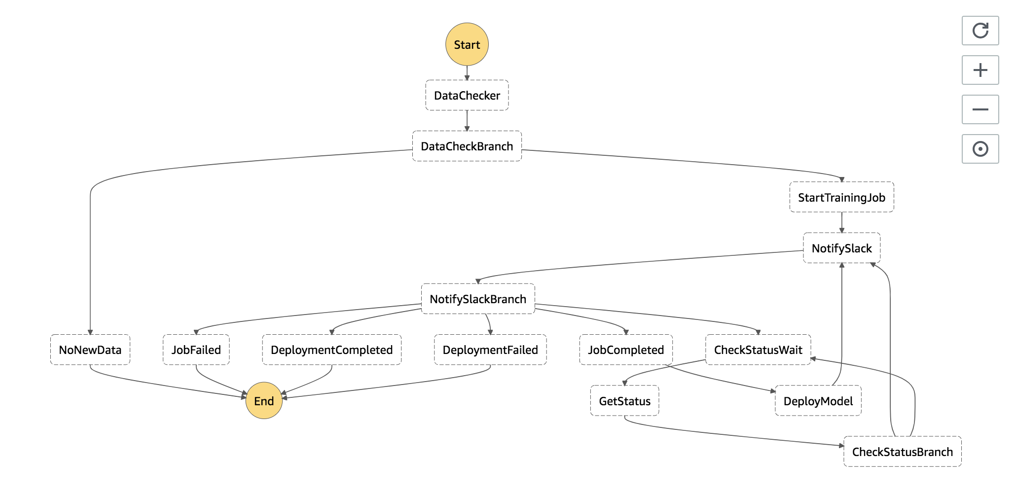
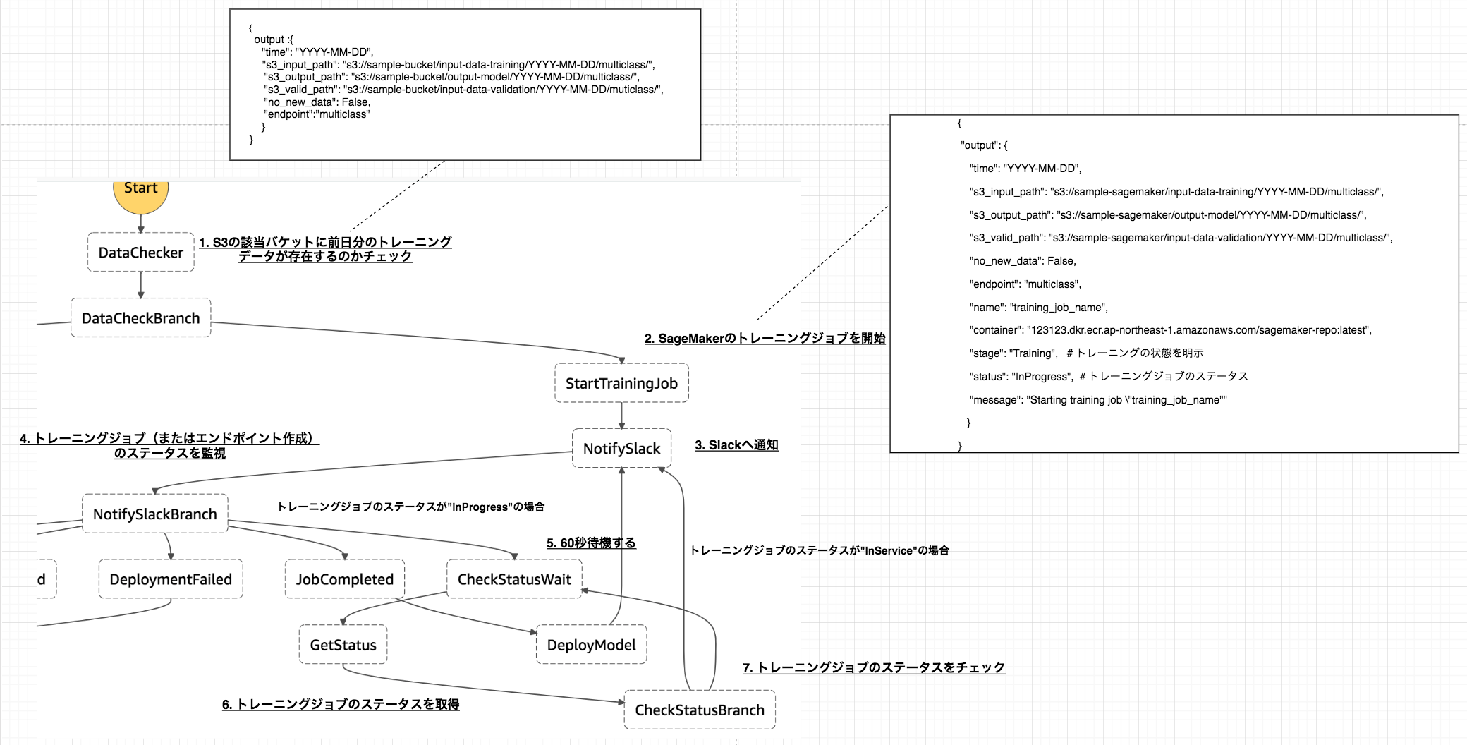
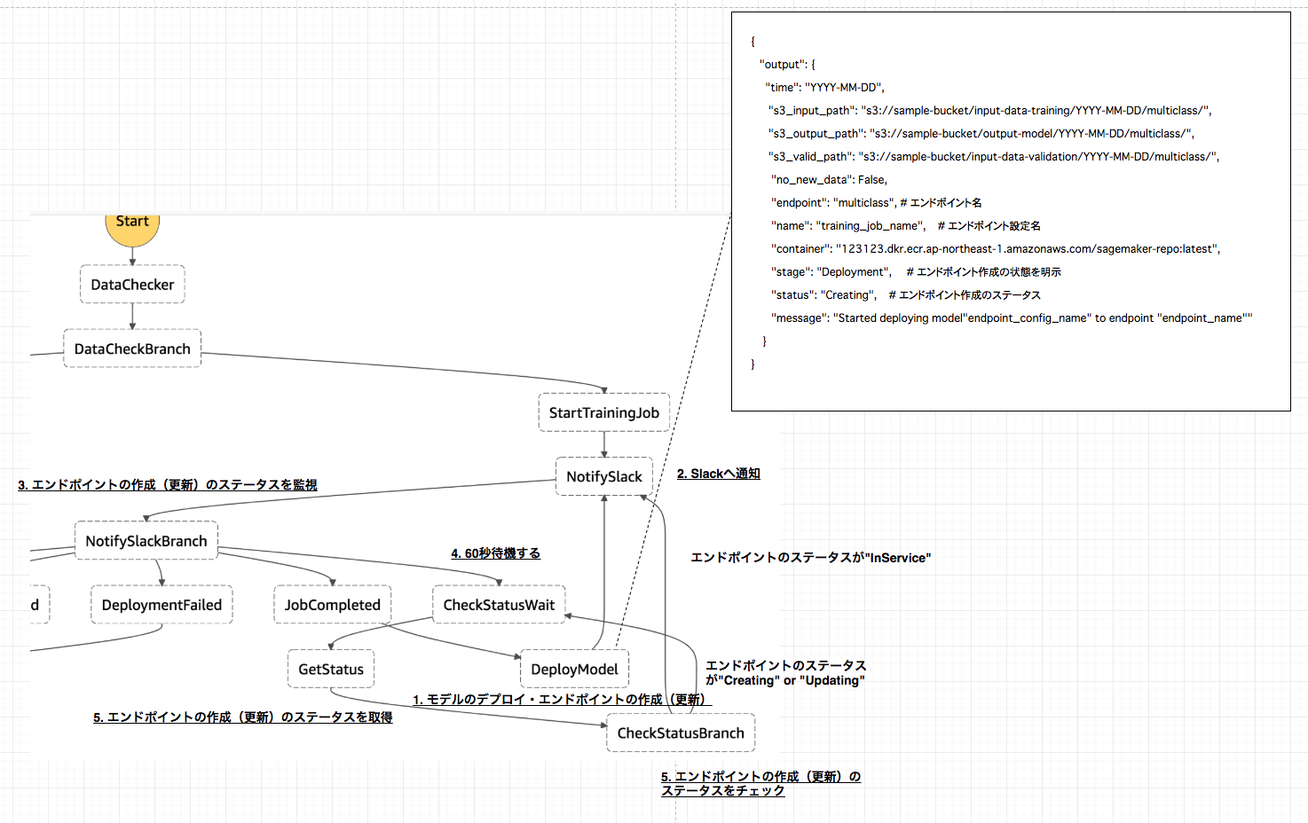
- 投稿日:2019-03-10T10:25:12+09:00
ネットワークの人間がNetmikoを試してみた
Netmikoとは?
"""""""""""""""
Netmikoとはネットワークデバイスとかにsshやtelnetで接続してなんやかやをやってくれるpythonのライブラリの一つらしい。
前身にParamikoとかいうものがあるらしいがtelnet接続に関するドキュメントをあまり拾えなかったので自分Paramikoあんまりわかんないです( ;∀;)使うきっかけ
"""""""""""""""
最近自分の仕事環境が変化し、ネットワークエンジニアなのに自動化とか触るようになりました。20台とか複数のデバイスに一人で設定投入とか手動でやっていたら残業三昧になって機器より先に人間壊れますよ....。ということでつまんない作業とか全部自動化したいなぁと思い最近netmikoとかautomationを勉強し始めています。なのでpythonの勉強自体も始めたのが少し前くらいになるのでプログラミングについてはズブの素人です。自分はもともとサポートの人なので基本的には機器で発生した不具合の検証とかしています。記事の目的
"""""""""""""""
Netmikoのライブラリでどんなことができるのか。というより自分ができるようになったのか。そちらの紹介です。
netmikoとかの勉強初めて2か月くらい?(正確には1か月とちょっと)のド素人でもこんなことができるよーになりましたという備忘録と
いやもっとこんな便利なことができるぞ!という知見を頂きたいという願望をもとにかいています。作ったもの
"""""""""""""""
簡単に言うと複数機器からバックアップのためにshow runをとってtxtファイルを作成し、ファイル名にタイムスタンプかいてます。devices.txtにはバックアップを取りたい機器のIPアドレスを入れてます。これで一つ一つのIPアドレスに接続して、show run 打ってtxtファイルに出してくれます。
一日の仕事の始めに検証に使う機器や設定しないといけない機器のバックアップとっとけという私の現場だと
このプログラムを起動している間にトイレいったり、コーヒーいれにいったりできるので大変便利になりました。#!/usr/bin/env python # -*- coding: utf-8 -*- from netmiko import ConnectHandler with open('devices.txt') as f: #一行ずつ読み込む devices = f.read().splitlines() for ip in devices: cisco_device = { 'device_type': 'なんでも_telnet',#telnet接続なら必須 'ip': ip, 'username': 'なんでも', 'password': 'なんでも', 'secret': 'なんでも', } print('Connecting to ' + ip) #ssh = connection ,telnet = net_connect net_connect = ConnectHandler(**cisco_device) print('Entering enable mode ...') net_connect.enable() output = net_connect.send_command('show run') prompt = net_connect.find_prompt() hostname = prompt[:-1] list = output.split('\n') list = list[3:] config = '\n'.join(list) import datetime #取得した日のタイムスタンプ now = datetime.datetime.now() today = str(now.year) + '-' + str(now.month) + '-' + str(now.day) file = today + '-' + hostname + '.txt' with open(file + '.txt', 'w') as backup: backup.write(config) print('Backup of ' + hostname + ' completed successfully') print('#' * 30) net_connect.disconnect()課題
このプログラム。自動でやってくれるのはいいんですが結構遅いんですよね(-_-メ)
手動でやるよりはだいぶ早いんですが、プログラムとしては遅いなぁという実感しかないです。所感
こんな感じで今後も自分の備忘録として残していきたいなぁと思ってます。