1. はじめに

2020年11月時点の TFLite Converter あるいは edgetpu compiler のどちらかにバグがあり、 TensorFlow v2.x の tf.image.resize オペレーションを含むモデルを量子化すると構造が壊れます。 下記に問題提起されています。

1. issue : Resize Nearest Neighbor does not convert #187 - google-coral/edgetpu
2. issue : Yolov4-Tiny EdgeTPU Missing Leaky Relu #51 - PINTO0309/PINTO_model_zoo
3. issue : RESIZE_NEAREST_NEIGHBOR Operation version not supported #42024 - tensorflow/tensorflow

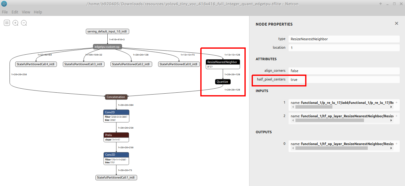
具体的には、下図の一例のようにEdgeTPUモデルへ変換した際の仕様不備により、 ResizeNearestNeighbor あるいは ResizeBilinear 以降の変換が正しく行われないばかりか、推論実行時に edgetpu_runtime が動作不安定になりエラーを出力します。 これは TensorFlow v1.x の頃には発生していなかった事象です。 half_pixel_centers が true の状態のモデルを量子化して生成すると発生します。 また、 EdgeTPUモデルへ変換せず INT8量子化 を行っただけのモデルの挙動も不安定になるなど、問題が多いです。

エラーの発生例は下記のとおりですが、 ResizeNearestNeighbor や ResizeBilinear の部分でエラーになるわけではなく、その後ろのどこかのレイヤーで仕様アンマッチによるエラーを引き起こしますので、問題の所在がとてもわかりくいバグです。

エラー例１

main.ERROR - Only float32 and uint8 is supported currently, got INT8.Node number 404 (LEAKY_RELU) failed to invoke.

エラー例２

main.ERROR - Only float32 and uint8 are supported currently, got -1695564548.Node number 5 (PRELU) failed to invoke.

2. 回避方法

下記は Cloud TPU を使用した場合に発生する類似の問題を回避する方法をご説明いただいている記事です。 今回は下記２種類の対処を同時に実施します。

1. TPUでアップサンプリングする際にエラーを出さない方法 - Shikoan's ML Blog - @koshian2さん
2. Colab TPUでもtensorflow.kerasでBilinear法のアップサンプリングを行う方法 - Qiita - @fwattyさん

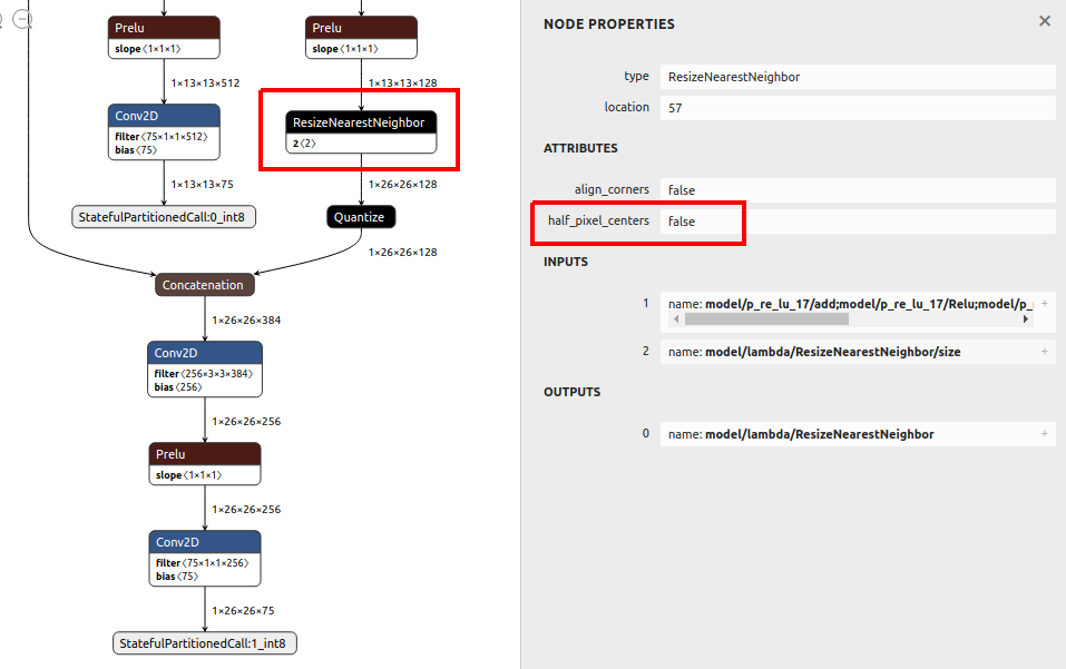
TensorFlow v1.x 世代の resize オペレーションへ置き換えることにより問題を回避します。 Lamda を経由してコールしないと Numpy 変換は対応していない、という旨のエラーが発生してしまいます。 Lamda でラップして定義した v1.x ベースの resize オペレーションは、正常に v2.x ベースの ResizeNearestNeighbor や ResizeBilinear へ変換されることを確認済みです。

Lamdaを使用したupsamplingの実装例

### 呼び出し先の関数定義 ############################################################
def upsampling2d_bilinear(x, upsampling_factor_height, upsampling_factor_width):
    w = x.shape[2] * upsampling_factor_width
    h = x.shape[1] * upsampling_factor_height
    return tf.compat.v1.image.resize_bilinear(x, (h, w))

def upsampling2d_nearest(x, upsampling_factor_height, upsampling_factor_width):
    w = x.shape[2] * upsampling_factor_width
    h = x.shape[1] * upsampling_factor_height
    return tf.compat.v1.image.resize_nearest_neighbor(x, (h, w))

### 呼び出し元のメインロジック #######################################################
# height方向に２倍、width方向に2倍のupsamplingを行います。整数のみ指定可能です。
x = Lambda(upsampling2d_bilinear,
           arguments={'upsampling_factor_height': 2,
                      'upsampling_factor_width':  2})(x)

# height方向に4倍、width方向に4倍のupsamplingを行います。整数のみ指定可能です。
x = Lambda(upsampling2d_nearest,
           arguments={'upsampling_factor_height': 4,
                      'upsampling_factor_width':  4})(x)

下図のように v1.x ベースの resize オペレーションを使用していても v2.x ベースの resize オペレーションへ正常に変換されていることが分かります。 更に half_pixel_centers が false に設定されていることが分かります。

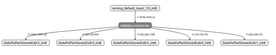
edgetpu_compiler を通して.tfliteをコンバートすると、下図のように全てのオペレーションが EdgeTPU 対応のカスタムオペレータに変換されたことが分かります。 これで EdgeTPU 上で推論を実行してもエラーになることはありません。

今回の問題を発生させる標準オペレーションは下記です。 そもそも half_pixel_centers を設定するパラメータがありませんので外から制御することができません。

• tf.image.resize https://www.tensorflow.org/api_docs/python/tf/image/resize

TF2.x_Resize_images_to_size_using_the_specified_method

tf.image.resize(
    images, size, method=ResizeMethod.BILINEAR, preserve_aspect_ratio=False,
    antialias=False, name=None
)

Args	Overview
images	4-D Tensor of shape [batch, height, width, channels] or 3-D Tensor of shape [height, width, channels].
size	A 1-D int32 Tensor of 2 elements: new_height, new_width. The new size for the images.
method	An image.ResizeMethod, or string equivalent. Defaults to bilinear.
preserve_aspect_ratio	Whether to preserve the aspect ratio. If this is set, then images will be resized to a size that fits in size while preserving the aspect ratio of the original image. Scales up the image if size is bigger than the current size of the image. Defaults to False.
antialias	Whether to use an anti-aliasing filter when downsampling an image.
name	A name for this operation (optional).

3. おわりに

以上です。 それでは皆さん、 良いTensorFlowライフを満喫してください！ ちなにみに私お手製の PyTorch(NCHW) to TensoFlow(NHWC) 変換ツール openvino2tensorflow はツールレベルで対処済みです。

はじめに

Kerasやtf.kerasのImageDataGeneratorは遅いので、tf.data.Datasetを使って学習を高速化してみます。
今回データ水増しにはKeras Preprocesing Layerを使用します。注：tensorflow2.3.0では使用可能ですが、まだ実験段階の機能とのことです。なのでご注意ください。

環境
python 3.6.9
tensorflow 2.3.0
GPU　GTX1060

参考文献

１．TensorFlow公式チュートリアル
チュートリアルらしく、step-by-stepでわかりやすいです。

２．TensorFlowで使えるデータセット機能が強かった話
tf.data.Datasetについてメチャクチャわかりやすい解説。とくにshuffleの説明がすごく良かったです。ありがとうございます。

３．scikit-learn、Keras、TensorFlowによる実践機械学習 第2版
第２版になってメチャクチャ厚くなりました、、、。これも良いです。

練習用データセットの準備

公式サイトに準じて、５種類の花の画像のデータセットをDLします。

python3

tf.keras.utils.get_file(origin='https://storage.googleapis.com/download.tensorflow.org/example_images/flower_photos.tgz',fname='flower_photos', untar=True)

Downloading data from https://storage.googleapis.com/download.tensorflow.org/example_images/flower_photos.tgz
228818944/228813984 [==============================] - 23s 0us/step
'/home/username/.keras/datasets/flower_photos'

上記によって下記のディレクトリに画像がDLされます。
/home/username/.keras/datasets/flower_photos

今回は予めtrainingとvalidationに画像を分けてしまい、trainingというディレクトリに９割、validationというディレクトリに１割の画像が収まるように分けます。
まずflower_photosの作業中のディレクトリにコピーしてください。

python3

import os
import shutil
import glob
import random

data_dir = './flower_photos'
directories = [i for i in glob.glob(os.path.join(data_dir, '*')) if os.path.isdir(i)]

directoriesには5つのディレクトリのパスが確認できます。
それぞれのディレクトリ名が画像のラベル（正解データ）になります。

python3

def make_dir(path):
    if not os.path.exists(path):
        os.mkdir(path)

train_dir = './training'
valid_dir = './validation'
make_dir(train_dir)
make_dir(valid_dir)

for i in directories:
    files = glob.glob(os.path.join(i, '*jpg'))
    random.seed(42)
    random.shuffle(files)
    train_dir = os.path.join(train_dir, os.path.basename(i))
    valid_dir = os.path.join(train_valid, os.path.basename(i))
    make_dir(train_dir)
    make_dir(valid_dir)
    for k in files[int(len(files)*0.9):]:
        shutil.move(k, train_dir)
    for k in files[:int(len(files)*0.9)]:
        shutil.move(k, valid_dir)

これで各ラベルの9割がtraining、1割がvalidationのフォルダにわけられました。

諸々importします。

python3

import tensorflow as tf
import numpy as np
import matplotlib.pyplot as plt
from PIL import Image
import random
AUTOTUNE = tf.data.experimental.AUTOTUNE

画像を収めたディレクトリを確認していきます。

python3

train_dir = './training'
valid_dir = './validation'
label_names = [os.path.basename(i) for i in glob.glob(os.path.join(train_dir, '*')) if os.path.isdir(i)]
label_names.sort()
print(label_names)

出力結果
['daisy', 'dandelion', 'roses', 'sunflowers', 'tulips']

daisy, dandelion, roses, sunflowers, tulipsの５つのラベルに別れています。余談ですが、このデータセット、何故か花以外の画像が混入しています。。。

画像の枚数を確認します。

python3

train_image_paths = glob.glob(os.path.join(train_dir, '*', '*jpg'))
valid_image_paths = glob.glob(os.path.join(valid_dir, '*', '*jpg'))
train_image_count = len(train_image_paths)
valid_image_count = len(valid_image_paths)
print('number of training image = ', train_image_count)
print('number of validation image = ', valid_image_count)

出力結果
number of training image =  3301
number of validation image =  369

Training画像が3301枚、Validation画像が369枚あります。

今度は、5つのラベルに任意のindex(番号)を割り付けます。どのように割り付けても良いと思います。

python3

label_to_index = dict((name, index) for index,name in enumerate(label_names))
label_to_index

出力結果
{'daisy': 0, 'dandelion': 1, 'roses': 2, 'sunflowers': 3, 'tulips': 4}

すべての画像pathに対してラベル付けを行いリストとして格納します。

python3

train_image_labels = [label_to_index[os.path.basename(os.path.dirname(path))]
                    for path in train_image_paths]
valid_image_labels = [label_to_index[os.path.basename(os.path.dirname(path))]
                    for path in valid_image_paths]

print("First 10 labels indices of train: ", train_image_labels[:10])
print("First 10 labels indices of validation: ", valid_image_labels[:10])

出力結果
First 10 labels indices of train:  [1, 1, 1, 1, 1, 1, 1, 1, 1, 1]
First 10 labels indices of validation:  [1, 1, 1, 1, 1, 1, 1, 1, 1, 1]

画像のpathはランダム化していないので、最初の10個をスライスすると、当然同じラベルになりました。

学習に向けてone-hot encodingする。

tf.one_hotを使用して、one-hot encodingします。5クラスですので、引数のdepthは5にします。

python3

train_image_labels = tf.one_hot(train_image_labels, depth=5)
valid_image_labels = tf.one_hot(valid_image_labels, depth=5)
print(train_image_labels[:10])

出力結果
tf.Tensor(
[[0. 1. 0. 0. 0.]
 [0. 1. 0. 0. 0.]
 [0. 1. 0. 0. 0.]
 [0. 1. 0. 0. 0.]
 [0. 1. 0. 0. 0.]
 [0. 1. 0. 0. 0.]
 [0. 1. 0. 0. 0.]
 [0. 1. 0. 0. 0.]
 [0. 1. 0. 0. 0.]
 [0. 1. 0. 0. 0.]], shape=(10, 5), dtype=float32)

順番が前後しましたが、画像を確認してみます。

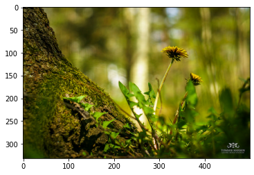
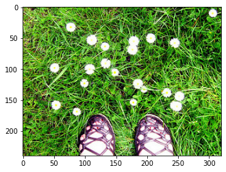
python3

img_path = train_image_paths[3]
img_raw = tf.io.read_file(img_path)
img_tensor = tf.image.decode_image(img_raw)#uint8にデコードしてtensor化
plt.imshow(img_tensor)

出力結果

＃画像の前処理関数を定義しておきます。
これはチュートリアルどおりです。

python3

def preprocess_image(image):
    image = tf.image.decode_jpeg(image, channels=3)#channelsは1だとGrayscale、3だとRGB
    image = tf.image.resize(image, [150, 150])
    image /= 255.0  #機械学習のためnormalizationします。
    return image

def load_and_preprocess_image(path):
    image = tf.io.read_file(path)
    return preprocess_image(image)

ようやくtf.data.Datasetを構築します。

さてここからが本題です。まず画像のpathをfrom_tensor_slicesを使用してtf.data.Dataset

python3

#まずtraining用画像のpathとlabelをそれぞれdataset化します。
path_ds = tf.data.Dataset.from_tensor_slices(train_image_paths)
label_ds = tf.data.Dataset.from_tensor_slices(train_image_labels)
#mapをつかってデータセット呼び出しに自動的に画像を変換するdatasetを作ります。
image_ds_train = path_ds.map(load_and_preprocess_image, num_parallel_calls=AUTOTUNE)
label_ds_train = tf.data.Dataset.from_tensor_slices(tf.cast(train_image_labels, tf.int64))

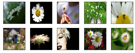
Datasetの挙動を確認がてら画像を確認します。

python3

plt.figure(figsize=(8,8))
for n, image in enumerate(image_ds_train.take(10)):
    plt.subplot(5, 5, n+1)
    plt.imshow(image)
    plt.grid(False)
    plt.xticks([])
    plt.yticks([])
    plt.grid(False)  
plt.show()

Datasetはイテレータとして動作し、image_ds_trainから.take(10)で10枚分の画像を呼び出しload_and_preprocess_imageによって画像サイズをリサイズ、正規化したものが返されます。
なおlabel_ds_trainはone-hot encodingされたラベルを返すイテレータとなります。

image_ds_trainとlabel_ds_trainは同じ順序ですので、zipすることで(image, label) というペアのデータセットができます。便利ですねー。

python3

image_label_ds_train = tf.data.Dataset.zip((image_ds_train, label_ds_train))
print(image_label_ds_train)

出力結果
<ZipDataset shapes: ((150, 150, 3), (5,)), types: (tf.float32, tf.int64)>

image_label_ds_trainはイテレータとして使用すると各iterationごとに画像とラベルの2つを返します。
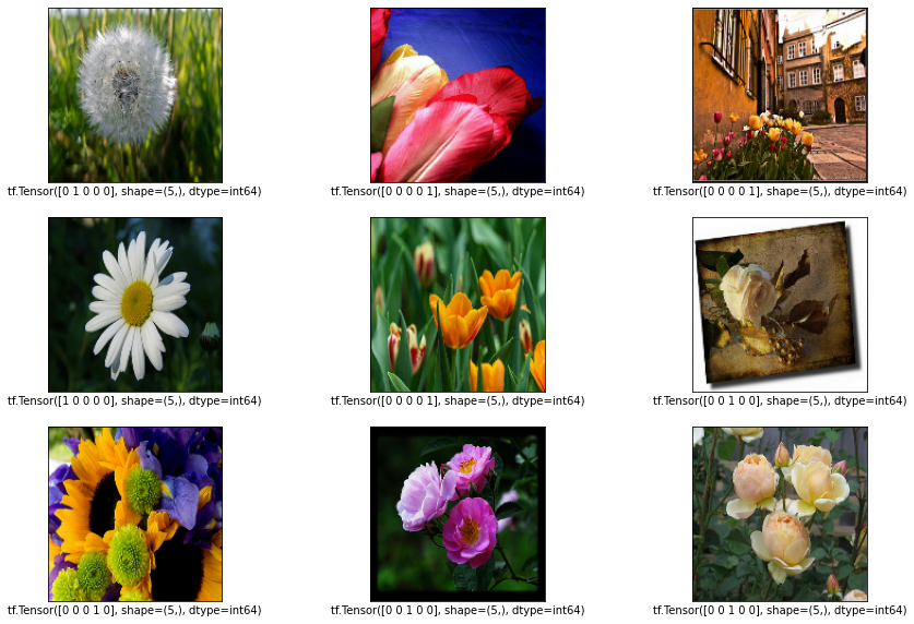
shuffle()については後述しますが、とりあえず挙動を確認してみます。

python3

plt.figure(figsize=(15,10))
for n,image in enumerate(image_label_ds_train.shuffle(train_image_count).take(9)):
    plt.subplot(3, 3, n+1)
    plt.imshow(image[0])
    plt.grid(False)
    plt.xticks([])
    plt.yticks([])
    plt.xlabel(os.path.basename(str(image[1])))  
    plt.grid(False)
plt.show()

出力結果。one-hot encodingされたラベルと画像が一致していることが確認できました。

さてパイプラインを完成させますが、ここでshuffle()について。
詳細は　TensorFlowで使えるデータセット機能が強かった話　を参考にしてください。
ポイントは
1.buffer_sizeはデータセットと同じ数にすることで、データが完全にシャッフルされます。
2.`.repeatの前に.shuffleすると1エポックの間に同じ画像が2回呼び出されるかもしれない。引用：TensorFlow公式チュートリアル

まずtrainingのジェネレーターを完成させます。

python3

BATCH_SIZE = 64

# シャッフルバッファのサイズをデータセットとおなじに設定することで、データが完全にシャッフルされる
# ようにできます。
ds = image_label_ds_train
ds = ds.repeat()
ds = ds.shuffle(buffer_size=train_image_count) #shuffleの順序注意！
ds = ds.batch(BATCH_SIZE)
ds = ds.prefetch(buffer_size=AUTOTUNE)
ds

validationも同様に作成しますが、validationはshuffleする必要はないので、shuffleなし。

python3

path_ds_valid = tf.data.Dataset.from_tensor_slices(valid_image_paths)
image_ds_valid = path_ds_valid.map(load_and_preprocess_image, num_parallel_calls=AUTOTUNE)
label_ds_valid = tf.data.Dataset.from_tensor_slices(tf.cast(valid_image_labels, tf.int64))
image_label_ds_valid = tf.data.Dataset.zip((image_ds_valid, label_ds_valid))

ds_valid = image_label_ds_valid
ds_valid = ds_valid.repeat()
ds_valid = ds_valid.batch(BATCH_SIZE)
ds_valid = ds_valid.prefetch(buffer_size=AUTOTUNE)
ds_valid

学習してみる。

適当にモデルを作成してコンパイルします。

python3

from tensorflow.keras.models import Sequential
from tensorflow.keras.layers import Dense, Conv2D, Flatten, Dropout, MaxPooling2D,BatchNormalization
from tensorflow.keras.preprocessing.image import ImageDataGenerator
IMG_HEIGHT = 150
IMG_WIDTH = 150
epochs = 20
model = Sequential([
    Conv2D(16, 3, padding='same', activation='relu', input_shape=(IMG_HEIGHT, IMG_WIDTH ,3)),
    BatchNormalization(),
    MaxPooling2D(),
    Conv2D(32, 3, padding='same', activation='relu'),
    BatchNormalization(),
    MaxPooling2D(),
    Conv2D(64, 3, padding='same', activation='relu'),
    BatchNormalization(),
    MaxPooling2D(),
    Dropout(0.5),
    Flatten(),
    Dense(512, activation='relu'),
    Dense(5, activation='softmax')
])

model.compile(optimizer='adam',
              loss='categorical_crossentropy',
              metrics=['accuracy'])

model.fitで学習します。kerasでよくお世話になったfit_generatorはもう使わないようです。
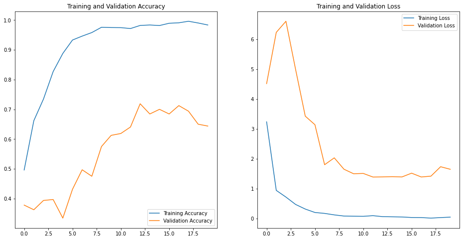
max_queue_size=120, workers=30, use_multiprocessing=True,の部分はお使いのcpuやosに合わせてください。

python3

history = model.fit(ds, 
        epochs=epochs, 
        steps_per_epoch=train_image_count//BATCH_SIZE,
        validation_data=ds_valid,
        validation_steps=valid_image_count//BATCH_SIZE, 
        validation_batch_size=BATCH_SIZE,
        max_queue_size=120, workers=30, use_multiprocessing=True,
        )

学習が始まります。

Epoch 1/20
 1/51 [..............................] - ETA: 0s - loss: 2.9178 - accuracy: 0.2656WARNING:tensorflow:Callbacks method `on_train_batch_end` is slow compared to the batch time (batch time: 0.0157s vs `on_train_batch_end` time: 0.0288s). Check your callbacks.
51/51 [==============================] - 2s 47ms/step - loss: 3.2386 - accuracy: 0.4960 - val_loss: 4.5163 - val_accuracy: 0.3781
・
・
・
Epoch 20/20
51/51 [==============================] - 2s 45ms/step - loss: 0.0474 - accuracy: 0.9835 - val_loss: 1.6496 - val_accuracy: 0.6438

結果をplotします。

python3

acc = history.history['accuracy']
val_acc = history.history['val_accuracy']

loss = history.history['loss']
val_loss = history.history['val_loss']

epochs_range = range(epochs)

plt.figure(figsize=(16, 8))
plt.subplot(1, 2, 1)
plt.plot(epochs_range, acc, label='Training Accuracy')
plt.plot(epochs_range, val_acc, label='Validation Accuracy')
plt.legend(loc='lower right')
plt.title('Training and Validation Accuracy')

plt.subplot(1, 2, 2)
plt.plot(epochs_range, loss, label='Training Loss')
plt.plot(epochs_range, val_loss, label='Validation Loss')
plt.legend(loc='upper right')
plt.title('Training and Validation Loss')
plt.show()

結果。過学習しているのか、training と　validationの曲線に乖離が見られました。

tf.data.Datasetにaugmentationを組み合わる。

TensorFlowの公式チュートリアルを参考にしました。
データの増強
Keras Preprocesing Layerを使用します。
注：tensorflow2.3.0では使用可能ですが、まだ実験段階の機能とのことです。

まず前処理レイヤーを作成します。

python3

data_augmentation = tf.keras.Sequential([
  tf.keras.layers.experimental.preprocessing.RandomFlip("horizontal_and_vertical"),
  tf.keras.layers.experimental.preprocessing.RandomRotation(0.2,fill_mode = 'reflect'),
  tf.keras.layers.experimental.preprocessing.RandomZoom(height_factor=0.2, fill_mode =  'reflect'),
])

1枚画像を使用して、水増しできているか確認します。

python3

#学習画像を1枚読み込みます。
img_path = train_image_paths[3]
img_raw = tf.io.read_file(img_path)
img_tensor = tf.image.decode_image(img_raw)#uint8にデコードしてtensor化
plt.imshow(img_tensor)

元画像

python3

img = tf.expand_dims(img_tensor, 0)
plt.figure(figsize=(10, 10))
for i in range(9):
    augmented_image = data_augmentation(img)
    ax = plt.subplot(3, 3, i + 1)
    plt.imshow(np.asarray(augmented_image[0], dtype=np.uint8))
    plt.axis("off")

どうやら水増しできているようです。
水増し手法は結構網羅されているようで、ここから確認できます。
水増ししたジェネレーターを作成します。

python3

ds_aug = image_label_ds_train
ds_aug = ds_aug.repeat()
ds_aug = ds_aug.shuffle(buffer_size=train_image_count) #shuffleの順序注意！
ds_aug = ds_aug.batch(BATCH_SIZE)
ds_aug = ds_aug.map(lambda x, y: (data_augmentation(x, training=True), y))
ds_aug = ds_aug.prefetch(buffer_size=AUTOTUNE)

モデルは先程と同じものを使用して学習しますが、重みを再利用してしまうので、新しく定義してコンパイルします。

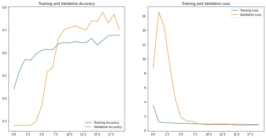
python3

model_aug = Sequential([
    Conv2D(16, 3, padding='same', activation='relu', input_shape=(IMG_HEIGHT, IMG_WIDTH ,3)),
    BatchNormalization(),
    MaxPooling2D(),
    Conv2D(32, 3, padding='same', activation='relu'),
    BatchNormalization(),
    MaxPooling2D(),
    Conv2D(64, 3, padding='same', activation='relu'),
    BatchNormalization(),
    MaxPooling2D(),
    Dropout(0.5),
    Flatten(),
    Dense(512, activation='relu'),
    Dense(5, activation='softmax')
])

model_aug.compile(optimizer='adam',
              loss='categorical_crossentropy',
              metrics=['accuracy'])

history = model_aug.fit(ds_aug, 
        epochs=epochs, 
        steps_per_epoch=train_image_count//BATCH_SIZE,
        validation_data=ds_valid,
        validation_steps=valid_image_count//BATCH_SIZE, 
        validation_batch_size=BATCH_SIZE,
        max_queue_size=120, workers=30, use_multiprocessing=True,
        )

学習結果

Epoch 1/20
51/51 [==============================] - 3s 55ms/step - loss: 3.3589 - accuracy: 0.4887 - val_loss: 11.0810 - val_accuracy: 0.2812
Epoch 2/20
51/51 [==============================] - 2s 46ms/step - loss: 1.1092 - accuracy: 0.5665 - val_loss: 16.0235 - val_accuracy: 0.2812
・
・
・
Epoch 20/20
51/51 [==============================] - 2s 47ms/step - loss: 0.7122 - accuracy: 0.7172 - val_loss: 0.6610 - val_accuracy: 0.7719

先ほどと同様に学習曲線をplotしてみると乖離が解消されており、データ水増しの効果が確認できました。

tf.data.Dataset＋Keras Preprocesing Layerとtf.kerasのflow+ImageDataGeneratorの速度比較

さて肝心の高速化はできてるのでしょうか？
同じ条件で旧来のtf.keras flow + ImageDataGeratorで学習を実行してみたところ、
1stepの速度
tf.data.Dataset : 46 - 48 msec
ImageDataGerator + flow : 65 - 69 msec
1epochの速度
tf.data.Dataset : 2 - 3 sec
ImageDataGerator + flow : 3 - 4 sec

と僅かながら高速化されています。僅かですが、もっと多量の画像を扱う場合はチリツモでしょう。
加えてtf.data.Datasetを使用した場合は、epoch間も早く全体的にはかなり高速化されているように感じます。

おわりに

まだ実験段階とのことですが、Keras Preprocesing Layerを使用して無事に水増しができました。はやく正式実装されるといいのですが・・・。tf.data.Datasetはとっつきにくいですが、なれればflow系の手法より高速に学習できますので、おすすめです！

はじめに

別記事で各種Data Augmentationを実装した際に、TensorFlow Addonsを使うと簡単にCutoutを実装できることに気づいた。
ここではDatasetに対してmap適用する実装とその評価を行う。

環境

• TensorFlow(2.3.0)
• tf.keras(2.4.0)
• tensorflow_addons(0.11.2)

Cutoutとは

画像のデータ拡張手法として提案されたもので、ランダムな座標の矩形を単色で塗りつぶす。
似たような手法にRandom Erasingがあるが、Cutoutのほうがより単純。
TensorFlow Addonsにはtfa.image.cutoutが用意されている。

実装

下記関数をDatasetのmap関数で適用する。

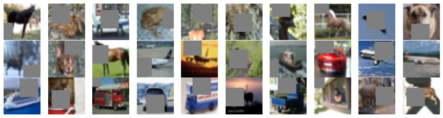
import tensorflow_addons as tfa
@tf.function
def cutout_augmentation(images, cutout_size, cval=0):
    img_shape = images.shape[-3:]
    mask_size = (int(img_shape[0]*cutout_size[0])//2*2, int(img_shape[1]*cutout_size[1])//2*2)
    images = tfa.image.random_cutout(images, mask_size, constant_values=cval)
    return images

cutout_sizeは塗りつぶす矩形のサイズを指定する。元画像からの比率を[H,W]としてfloatで指定する。32x32画像の場合は[0.5,0.5]で16x16の範囲を塗りつぶす。
cvalは塗りつぶす色。0.0～1.0の画像の場合はcval=0.5で灰色となる。

tensorflow-addonsのバージョンが古いと使えないので、Google Colabでは!pip install --upgrade tensorflow-addonsを事前に実行する。

実行結果はこちら。

評価

矩形サイズの設定値の影響や、他のAugmentationとの比較を行う。

• Google ColabのTPUでCIFAR10の学習を3回行い、ValidationのAccuracyの中間値で比較
• Vertical Flipのみ使用したものをベースとして、そこに以下のAugmentation処理を追加して実施
  • Cutout(0.4～0.8)
  • Width/Height Shift (range=0.25,fill_mode='constant'および'reflect' )
  • Cutout + Width/Height Shift('reflect')
• SGD(lr=0.01/momentum=0.9)で100epoch、100～150epochはlr=0.001に変更

結果はこちら。

拡張法	cutout	fill_mode	Accuracy
Vertical Flip	-	-	89.15
Cutout	0.4	-	91.80
Cutout	0.5	-	92.31
Cutout	0.6	-	92.50
Cutout	0.7	-	92.63
Cutout	0.8	-	92.53
Shift	-	constant	92.86
Shift	-	reflect	93.39
Cutout+Shift	0.5	reflect	94.43

Cutoutのサイズ比較では0.7が最も良好だった。0.7*0.7=0.49なので、ほぼ半分が消えることになる。
元論文ではCIFAR10では16x16つまり0.5が最も良いとされていたので結果にはずれがあった。モデルの違いが影響しているのか？。
同論文ではCIFAR100の場合はもっとサイズを下げたほうが好結果となっている。学習内容によってパラメータ調整する余地があるようだ。
Shiftとの比較になると、Shiftのほうが好結果だった。
全体としては、ShiftとCutoutを混ぜたものが最も好結果となった。Shift(reflect)からは1%の認識率向上があるが、このレベルでは結構大きな差なので同時に適用する価値は十分あると思われる。

実験用コードはこちら。

参考

ImageDataGeneratorを拡張しcutoutを実装する
PyTorchでデータ水増し（Data Augmentation）する方法