はじめに

Keras の Functional API を使った基本的なモデルの実装と多入力・多出力モデルを実装する方法について紹介します。

環境

今回は Tensorflow に統合された Keras を利用しています。

tensorflow==2.3.0

ゴール

• Functional API が使える
• 多入力・多出力モデルを実装できる

Functional API とは

Sequential モデルより柔軟なモデルを実装できるものになります。
今回は、Sequential モデルでは表現できないモデルの中から多入力・多出力モデルを実装していきます。

基本的な使い方

まずは、Functional API の基本的な使い方を説明していきます。
Functional API はモデルを定義する方法なので、学習・評価・予測は Sequential モデルと同じになります。

入力層

まずは、keras.Inputで入力層を定義します。

inputs = keras.Input(shape=(128,))

中間層・出力層

以下のように層を追加していくことができ、最後の層が出力層になります。

x = layers.Dense(64, activation="relu")(inputs)
outputs = layers.Dense(10)(x)

モデル作成

層の定義が完了したら、入力層と出力層を指定して、モデルを作成します。

model = keras.Model(inputs=inputs, outputs=outputs, name="model")

Sequential モデルとの比較

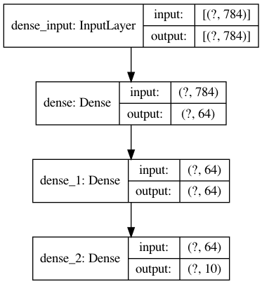
Sequential モデルと Functional API で同じモデルを実装してみます。

実装するモデルは以下の通りです。

Sequential モデル

from tensorflow import keras
from tensorflow.keras import layers
from tensorflow.keras.models import Sequential

model = Sequential()
model.add(layers.Dense(64, activation='relu', input_shape=(784,)))
model.add(layers.Dense(64, activation='relu'))
model.add(layers.Dense(10, activation='softmax'))

Functional API

from tensorflow import keras
from tensorflow.keras import layers

inputs = keras.Input(shape=(784,))
x = layers.Dense(64, activation='relu')(inputs)
x = layers.Dense(64, activation='relu')(x)
outputs = layers.Dense(10, activation='softmax')(x)
model = keras.Model(inputs=inputs, outputs=outputs)

多入力・多出力モデル

Functional API で多入力・多出力モデルを実装していきます。

多入力

入力層を複数定義することで、多入力にすることができます。
複数の層をまとめるときは、layers.concatenateを利用します。

inputs1 = keras.Input(shape=(64,), name="inputs1_name")
inputs2 = keras.Input(shape=(32,), name="inputs2_name")

x = layers.concatenate([inputs1, inputs2])

多出力

中間層を複数に渡すことで、層を分岐させることができます。
終点となる層が複数になることで、多出力になります。

outputs1 = layers.Dense(64, name="outputs1_name")(x)
outputs2 = layers.Dense(32, name="outputs2_name")(X)

コンパイル

複数の出力層がある場合は、それぞれに損失関数と重みを指定できます。

model.compile(
    optimizer=keras.optimizers.RMSprop(1e-3),
    loss={
        "outputs1_name": keras.losses.BinaryCrossentropy(from_logits=True),
        "outputs2_name": keras.losses.CategoricalCrossentropy(from_logits=True),
    },
    loss_weights=[1.0, 0.5],
)

学習

層につけた名前で入力データと出力データ（ターゲット）を指定して、学習させることができます。

model.fit(
    {"inputs1_name": inputs1_data, "inputs2_name": inputs2_data},
    {"outputs1_name": outputs1_targets, "outputs2_name": outputs2_targets},
    epochs=2,
    batch_size=32,
)

具体例

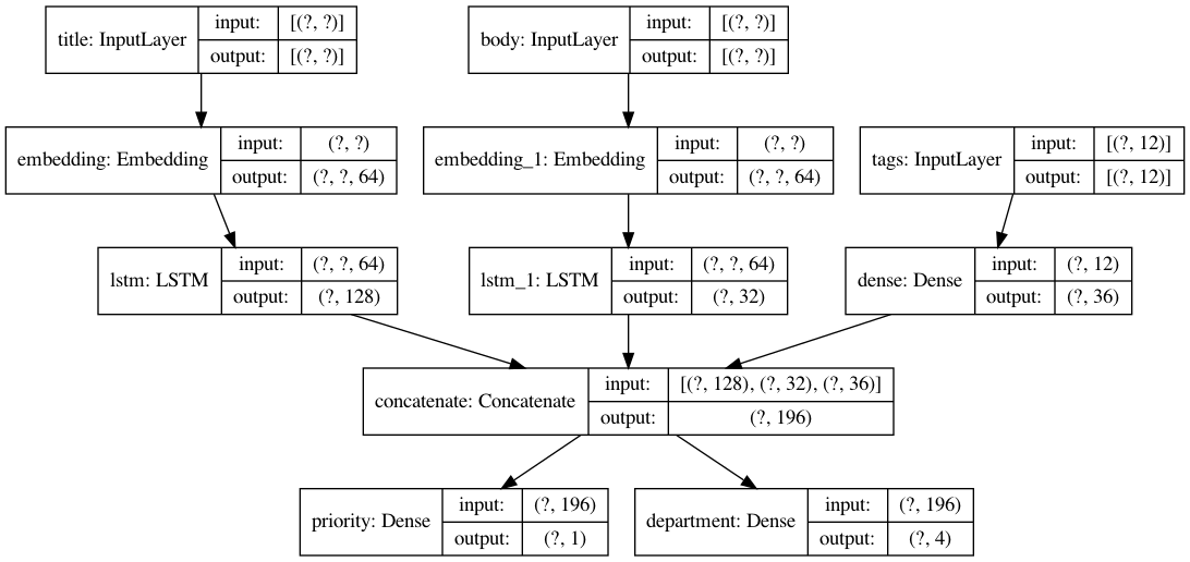
具体的な例を用いて実装してきます。

ここでは、顧客からの問い合わせのタイトルと本文とタグから、その問い合わせの優先度と対応部門を予測します。

入力

• タイトル
• 本文
• タグ

出力

• 優先度
• 対応部門

from tensorflow import keras
from tensorflow.keras import layers
import numpy as np

num_tags = 12
num_words = 10000
num_departments = 4

# ダミーデータの作成
title_data = np.random.randint(num_words, size=(1280, 10))
body_data = np.random.randint(num_words, size=(1280, 100))
tags_data = np.random.randint(2, size=(1280, num_tags)).astype("float32")
priority_targets = np.random.random(size=(1280, 1))
dept_targets = np.random.randint(2, size=(1280, num_departments))

# タイトルの層
title_input = keras.Input(
    shape=(None,), name="title"
)
title_features = layers.Embedding(num_words, 64)(title_input)
title_features = layers.LSTM(128)(title_features)

# 本文の層
body_input = keras.Input(shape=(None,), name="body")
body_features = layers.Embedding(num_words, 64)(body_input)
body_features = layers.LSTM(32)(body_features)

# タグの層
tags_input = keras.Input(
    shape=(num_tags,), name="tags"
)
tags_features = layers.Dense(36, activation='relu')(tags_input)

# 層を結合
x = layers.concatenate([title_features, body_features, tags_features])

# 出力層
priority_output = layers.Dense(1, name="priority")(x)
department_output = layers.Dense(num_departments, name="department")(x)

model = keras.Model(
    inputs=[title_input, body_input, tags_input],
    outputs=[priority_output, department_output],
)

# モデルをコンパイル
model.compile(
    optimizer=keras.optimizers.RMSprop(1e-3),
    loss={
        "priority": keras.losses.BinaryCrossentropy(from_logits=True),
        "department": keras.losses.CategoricalCrossentropy(from_logits=True),
    },
    loss_weights=[1.0, 0.5],
)

# 学習
model.fit(
    {"title": title_data, "body": body_data, "tags": tags_data},
    {"priority": priority_targets, "department": dept_targets},
    epochs=2,
    batch_size=32,
)

まとめ

• Functional API を使うと多入力・多出力のモデルを実装できる

参考文献

• Keras Functional API  |  TensorFlow Core
• Python と Keras によるディープラーニング

Qrunchのサービス終了に伴い転記

---

title: 線形回帰問題をディープラーニングで解く
tags: TensorFlow
categories:
author: @glowflowplow
status: public
created_at: 2018-11-30 18:21:00 +0900
updated_at: 2018-12-01 08:41:36 +0900
published_at: 2018-11-30 18:21:00 +0900

---

目的

TensorFlowの扱い方を学ぶ

問題

y = 2 * x + 1

を与えられたxから求める

環境

• OS : MacOS
• 言語 : Python2.7
• ライブラリ : TensorFlow

環境に関する知識がないので細かい所はわかりません

回答

あらすじ

• データセットの作成
• 推定ロジックの設計
• 損失の設計
• 学習手法の指定
• 学習の実行
• 精度の検証
• 学習モデルの保存
• 別のスクリプトから学習モデルを利用する

上記を踏まえて作成したコード

とりあえず全体のコード貼ったほうがいいかなと．下で各関数の説明をする

import tensorflow as tf
import sys
import numpy as np

BATCH_SIZE = 100
TRAIN_STEP = 100

def main():
    x_data, y_data = generate(BATCH_SIZE * TRAIN_STEP)
    x_test, y_test = generate(BATCH_SIZE)

    x = tf.placeholder('float32', shape=(None, 1))
    y_= tf.placeholder('float32', shape=(None, 1))

    logits = inference(x)
    loss = loss_function(logits, y_)
    train_op = training(loss)
    accuracy = accuracy_function(logits, y_)

    saver = tf.train.Saver()
    sess = tf.Session()
    sess.run(tf.global_variables_initializer())

    for step in range(TRAIN_STEP):
        for i in range(BATCH_SIZE):
            batch = BATCH_SIZE * i
            sess.run(train_op, feed_dict={
                x : x_data[batch:batch+BATCH_SIZE],
                y_: y_data[batch:batch+BATCH_SIZE]
                })

        train_accuracy = sess.run(accuracy, feed_dict={
            x : x_data,
            y_: y_data
            })
        print "step%d, accuracy %g"%(step, train_accuracy)

    print "test accuracy %g" %sess.run(accuracy, feed_dict={
        x : x_test,
        y_: y_test
        })
    saver.save(sess, "./checkpoint/sample_model.ckpt")

def generate(size):
    x = [[np.random.random()] for i in range(size)]
    y = [[function(x[i][0])] for i in range(size)]
    return x, y

def function(x):
    return float(2*x+1)

def inference(x_ph):
    w = tf.Variable(tf.random_normal([1, 1], dtype=tf.float32))
    b = tf.Variable(tf.constant(0, 'float32', [1]))
    y = tf.nn.relu(x_ph * w + b)
    return y

def loss_function(y, y_):
    return tf.math.pow(tf.cast(y - y_, tf.float32), 2)

def training(loss):
    return tf.train.AdamOptimizer(0.001).minimize(loss)

def accuracy_function(y, y_):
    return tf.reduce_mean(tf.cast(tf.less(tf.abs(tf.subtract(y , y_)), 0.01), 'float'))



if __name__ == '__main__':
    main()

データセットの作成

def generate(size):
    x = [[np.random.random()] for i in range(size)]
    y = [[function(x[i][0])] for i in range(size)]
    return x, y

def function(x):
    return float(2*x+1)

xの定義域は(0<=x<=1)
yの値域は(1<=y<=3)
floatを指定しているのはTensorFlowが型にうるさいから．
なぜ必要なのかは理解していない．

推定ロジックの設計

def inference(x_ph):
    w = tf.Variable(tf.random_normal([1, 1], dtype=tf.float32))
    b = tf.Variable(tf.constant(0, 'float32', [1]))
    y = tf.nn.relu(x_ph * w + b)
    return y

tf.Variable()はTensorFlow上での変数宣言のようなもの．これが学習訓練によって変化する
その他関数の動作についてはリファレンスを読んで

ニューラルネットワークの設計

この問題の本題でないのであからさまに適当．
x = [a]
w = [b c]^T
b = [d]
y = [a] * [b c] + [d] = ab + ac + d

となるはず

tf.nn.relu()関数を使用する理由

深層学習でなんかよく使われる．理由は他所で色々解説されているのでそちらを参照して．この問題に対しては使わない方が良い結果が得られると思うが、それは答えを知ってるから言えることだからと考えておく

損失の設計

def loss_function(y, y_):
    return tf.math.pow(tf.cast(y - y_, tf.float32), 2)

二乗誤差．と言っても要素が一つしかないので差の二乗．ここでfloatを指定しないと怒られる．

学習手法の指定

def training(loss):
    return tf.train.AdamOptimizer(0.001).minimize(loss)

Q.AdamOptimizerって何ですか？？？
A.Adamアルゴリズムを実装したオプティマイザ
なんかよくわからないけど優秀らしい．深層学習の設計者になるならこれを含めてオプティマイザに実装されているアルゴリズムを理解しておいた方がいいと思う．今回の本題ではないのでスルーするー

学習の実行

    sess = tf.Session()
    sess.run(tf.global_variables_initializer())

    for step in range(TRAIN_STEP):
        for i in range(BATCH_SIZE):
            batch = BATCH_SIZE * i
            sess.run(train_op, feed_dict={
                x : x_data[batch:batch+BATCH_SIZE],
                y_: y_data[batch:batch+BATCH_SIZE]
                })

この辺のこと
セッションの初期化にはtf.initialize_all_variables()を最初は指定していたが、コンパイラにこれを使えと言われてtf.global_variables_initializer()になった．よくわからない．
どうやら以前の関数は廃止されたらしい

精度の検証

    for step in range(TRAIN_STEP):
        for i in range(BATCH_SIZE):
　　# 中略
        train_accuracy = sess.run(accuracy, feed_dict={
            x : x_data,
            y_: y_data
            })
        print "step%d, accuracy %g"%(step, train_accuracy)

    print "test accuracy %g" %sess.run(accuracy, feed_dict={
        x : x_test,
        y_: y_test
        })

ここと

def accuracy_function(y, y_):
    return tf.reduce_mean(tf.cast(tf.less(tf.abs(tf.subtract(y , y_)), 0.01), 'float'))

この部分
精度を、バッチの中の推定値と正答の差が0.01以下の要素の割合に指定
これをバッチ分訓練する毎と全ての訓練が終わったあとに実行．出力は

$ python sample.py
2018-11-20 21:33:47.419183: I tensorflow/core/platform/cpu_feature_guard.cc:141] Your CPU supports instructions that this TensorFlow binary was not compiled to use: AVX2 FMA
step0, accuracy 0
step1, accuracy 0
step2, accuracy 0
step3, accuracy 0
step4, accuracy 0
step5, accuracy 0
step6, accuracy 0
step7, accuracy 0
step8, accuracy 0
step9, accuracy 0
step10, accuracy 0
step11, accuracy 0
step12, accuracy 0
step13, accuracy 0
step14, accuracy 0
step15, accuracy 0
step16, accuracy 0
step17, accuracy 0.0646
step18, accuracy 0.1448
step19, accuracy 0.1622
step20, accuracy 0.1743
step21, accuracy 0.1852
step22, accuracy 0.1922
step23, accuracy 0.2017
step24, accuracy 0.2113
step25, accuracy 0.227
step26, accuracy 0.2386
step27, accuracy 0.2465
step28, accuracy 0.2584
step29, accuracy 0.2689
step30, accuracy 0.2797
step31, accuracy 0.2912
step32, accuracy 0.3026
step33, accuracy 0.3164
step34, accuracy 0.3303
step35, accuracy 0.3459
step36, accuracy 0.3629
step37, accuracy 0.3807
step38, accuracy 0.4021
step39, accuracy 0.4255
step40, accuracy 0.4494
step41, accuracy 0.4772
step42, accuracy 0.5113
step43, accuracy 0.5506
step44, accuracy 0.5906
step45, accuracy 0.6354
step46, accuracy 0.6866
step47, accuracy 0.7514
step48, accuracy 0.8233
step49, accuracy 0.8973
step50, accuracy 0.9429
step51, accuracy 0.9967
step52, accuracy 1
step53, accuracy 1
step54, accuracy 1
step55, accuracy 1
step56, accuracy 1
step57, accuracy 1
step58, accuracy 1
step59, accuracy 1
step60, accuracy 1
step61, accuracy 1
step62, accuracy 1
step63, accuracy 1
step64, accuracy 1
step65, accuracy 1
step66, accuracy 1
step67, accuracy 1
step68, accuracy 1
step69, accuracy 1
step70, accuracy 1
step71, accuracy 1
step72, accuracy 1
step73, accuracy 1
step74, accuracy 1
step75, accuracy 1
step76, accuracy 1
step77, accuracy 1
step78, accuracy 1
step79, accuracy 1
step80, accuracy 1
step81, accuracy 1
step82, accuracy 1
step83, accuracy 1
step84, accuracy 1
step85, accuracy 1
step86, accuracy 1
step87, accuracy 1
step88, accuracy 1
step89, accuracy 1
step90, accuracy 1
step91, accuracy 1
step92, accuracy 1
step93, accuracy 1
step94, accuracy 1
step95, accuracy 1
step96, accuracy 1
step97, accuracy 1
step98, accuracy 1
step99, accuracy 1
test accuracy 1

なんでバッチサイズが100なのに小数点以下3桁が変動してるのか．どこかに問題がありそう
サンプルを100個ずつ100step学習した結果、52回目から訓練の精度が1になり、学習後のテストでも1が得られた．精度がよくなるタイミングはよくブレて運が悪いと100stepでは足りないことがある．

学習モデルの保存

せっかく訓練しても訓練後のモデルを使えなくては意味がない．よって
学習モデルを保存する必要があるので、訓練の前にsaver = tf.train.Saver()
と訓練後にsaver.save(sess, "./checkpoint/sample_model.ckpt")を入れる．
./checkpointディレクトリは予め用意しておく必要がある．
これを入れて実行すると保存したディレクトリに下のファイルとディレクトリが得られる．

$ ls checkpoint/
checkpoint              sample_model.ckpt.index
sample_model.ckpt.data-00000-of-00001   sample_model.ckpt.meta

直感的にsample_model.ckptが存在しないのは違和感があるが、読み込む際はsample_model.ckptを指定する．意味わからん

別のスクリプトから学習モデルを利用する

import tensorflow as tf
import numpy as np

def main():
    x = tf.placeholder('float32', shape=(None, 1))
    logits = inference(x)
    sess = tf.InteractiveSession()

    saver = tf.train.Saver()
    sess.run(tf.initialize_all_variables())
    saver.restore(sess, "./checkpoint/sample_model.ckpt")

    x_data = [[0.1*i] for i in range(11)]
    print x_data

    estimate_data = logits.eval({x: x_data})
    print estimate_data

    x_data = [[0.1*i+1] for i in range(10)]
    estimate_data = logits.eval({x: x_data})
    print np.round(x_data, 3)
    print np.round(estimate_data, 3)


def inference(x_ph):
    w = tf.Variable(tf.random_normal([1, 1], dtype=tf.float32))
    b = tf.Variable(tf.constant(0, 'float32', [1]))
    y = tf.nn.relu(x_ph * w + b)
    return y



main()

どうやらニューラルネットワークの設計は同じものを用意しなくてはいけない模様．
logitsに同じNNを用意．Sessionは対話的セッションを用意．

saver.restore(sess, "./checkpoint/sample_model.ckpt")

で学習モデルの読み込み．
logits.eval()はセッション内でテンソルで値を評価する．
ちょっとよくわからないところが多いが、これで学習モデルに値を入力できる．
入力は訓練でのxの定義域(0<=x<=1)内を0.1刻みと、1から2まで同じく0.1刻み．
結果は

[[0.0], [0.1], [0.2], [0.30000000000000004], [0.4], [0.5], [0.6000000000000001], [0.7000000000000001], [0.8], [0.9], [1.0]]
[[1.000003 ]
 [1.2000024]
 [1.400002 ]
 [1.6000015]
 [1.8000009]
 [2.0000005]
 [2.1999998]
 [2.3999991]
 [2.599999 ]
 [2.7999983]
 [2.9999976]]
[[1. ]
 [1.1]
 [1.2]
 [1.3]
 [1.4]
 [1.5]
 [1.6]
 [1.7]
 [1.8]
 [1.9]]
[[3. ]
 [3.2]
 [3.4]
 [3.6]
 [3.8]
 [4. ]
 [4.2]
 [4.4]
 [4.6]
 [4.8]]

となった．

最後に

これで線形回帰問題を深層学習を用いて解けた.
と言っていいのかわからないが、きっと解けたんだろう.
「なぜかはわからない」「理解していない」「理解しておいたほうがいいだろう」と後回しにしたことが多いのでこの辺の知識をちゃんと調べて補完したほうがいいのだろうなと.
間違っているところ等あったらご指摘ください。

Word2vecを使ってみる

・word2vecを使うためにgensimのインストールをする。
・文字処理をするためにjanomeをインストールする。

pip install gensim
pip install janome

・word2vecで青空文庫を読み込むためのコード

//必要なライブラリのインポート

from janome.tokenizer import Tokenizer
from gensim.models import word2vec
import re

//txtファイルをopenした後読む
binarydata = open("kazeno_matasaburo.txt).read()

ーーーーーーーーーーーーーーーーーーーーーーーーーーーーーーーーーーーーーーー
//ちなみにprintして一つ一つ確かめたやつ

binarydata = open("kazeno_matasaburo.txt)
print(type(binarydata))
実行結果　　<class '_io.BufferedReader'>
binarydata = open("kazeno_matasaburo.txt).read()
print(type(binarydata))
実行結果　<class 'bytes'>
ーーーーーーーーーーーーーーーーーーーーーーーーーーーーーーーーーーーーーーー
//データ型を文字列型に変換（pythonの書き方）
text = binarydata.decode('shift_jis')
//いらないデータを削ぎ落とす
text = re.split(r'\-{5,}',text)[2]
text = re.split(r'底本：',text)[0]
text = text.strip()

//形態素解析を行う
t = Tokenizer()
results = []
lines = text.split("\r\n") //行ごとに分けられている

for line in lines:
    s = line
    s = s.replace('|','')
    s = re.sub(r'《.+?》','',s)
    s = re.sub(r'［＃.+?］','',s)
    tokens = t.tokenize(s) //解析したやつが入っている
    r = []
　　//一つずつ取り出して、.base_formとか.surfaceとかでアクセスできる
    for token in tokens:
        if token.base_form == "*":
            w = token.surface
        else:
            w = token.base_form
        ps = token.part_of_speech
        hinshi = ps.split(',')[0]
        if hinshi in ['名詞','形容詞','動詞','記号']:
            r.append(w)
    rl = ("　".join(r)).strip()
    results.append(rl)
    print(rl)

//解析したやつを書き込むファイルの生成と同時に書き込む
wakachigaki_file = "matasaburo.wakati"
with open(wakachigaki_file,'w', encoding='utf-8') as fp:
    fp.write('\n'.join(results))

//解析スタート
data = word2vec.LineSentence(wakachigaki_file)
model = word2.Word2Vec(data,size=200,window=10,hs=1,min_count=2,sg=1)
model.save('matasaburo.model')

//model使ってみる
model.most_similar(positive=['学校'])

まとめ

①解析したい文章を取ってくる。
②文章だけになるように加工する。最後の参考文献みたいなやつとか取り除く
③for文で１行ずつ取り出して、いらない部分を取り除く。
④tokenizerで形態素解析をする。リストに入れる。
⑤作ったリストをファイルに書き込む
⑥形態素解析したファイルを使ってmodelを作る

Word2vecを使ってみる

・word2vecを使うためにgensimのインストールをする。
・文字処理をするためにjanomeをインストールする。

pip install gensim
pip install janome

・word2vecで青空文庫を読み込むためのコード

//必要なライブラリのインポート

from janome.tokenizer import Tokenizer
from gensim.models import word2vec
import re

//txtファイルをopenした後読む
binarydata = open("kazeno_matasaburo.txt).read()

ーーーーーーーーーーーーーーーーーーーーーーーーーーーーーーーーーーーーーーー
//ちなみにprintして一つ一つ確かめたやつ

binarydata = open("kazeno_matasaburo.txt)
print(type(binarydata))
実行結果　　<class '_io.BufferedReader'>
binarydata = open("kazeno_matasaburo.txt).read()
print(type(binarydata))
実行結果　<class 'bytes'>
ーーーーーーーーーーーーーーーーーーーーーーーーーーーーーーーーーーーーーーー
//データ型を文字列型に変換（pythonの書き方）
text = binarydata.decode('shift_jis')
//いらないデータを削ぎ落とす
text = re.split(r'\-{5,}',text)[2]
text = re.split(r'底本：',text)[0]
text = text.strip()

//形態素解析を行う
t = Tokenizer()
results = []
lines = text.split("\r\n") //行ごとに分けられている

for line in lines:
    s = line
    s = s.replace('|','')
    s = re.sub(r'《.+?》','',s)
    s = re.sub(r'［＃.+?］','',s)
    tokens = t.tokenize(s) //解析したやつが入っている
    r = []
　　//一つずつ取り出して、.base_formとか.surfaceとかでアクセスできる
    for token in tokens:
        if token.base_form == "*":
            w = token.surface
        else:
            w = token.base_form
        ps = token.part_of_speech
        hinshi = ps.split(',')[0]
        if hinshi in ['名詞','形容詞','動詞','記号']:
            r.append(w)
    rl = ("　".join(r)).strip()
    results.append(rl)
    print(rl)

//解析したやつを書き込むファイルの生成と同時に書き込む
wakachigaki_file = "matasaburo.wakati"
with open(wakachigaki_file,'w', encoding='utf-8') as fp:
    fp.write('\n'.join(results))

//解析スタート
data = word2vec.LineSentence(wakachigaki_file)
model = word2.Word2Vec(data,size=200,window=10,hs=1,min_count=2,sg=1)
model.save('matasaburo.model')

//model使ってみる
model.most_similar(positive=['学校'])

まとめ

①解析したい文章を取ってくる。
②文章だけになるように加工する。最後の参考文献みたいなやつとか取り除く
③for文で１行ずつ取り出して、いらない部分を取り除く。
④tokenizerで形態素解析をする。リストに入れる。
⑤作ったリストをファイルに書き込む
⑥形態素解析したファイルを使ってmodelを作る

データセットづくりに

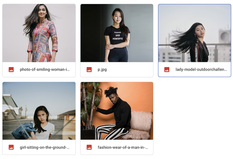
フォルダ内の画像を一気に切り抜けるノートブックをつくりました。
TensorFlow公式のDeepLabのノートブックが元になっています。

使い方

1,ノートブックを開く。

2,ご自身のGoogle Driveに切り抜きたい画像のフォルダをアップロード。保存先フォルダも作る。

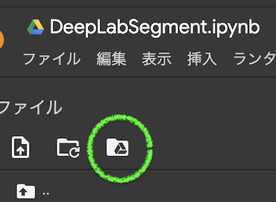
3,ノートブックからGoogle Driveをマウント

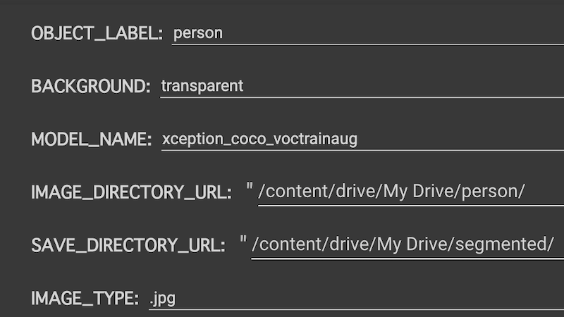
4,メニューから、切り抜きたいオブジェクト、背景モード、使用したいモデル、画像フォルダのパス、保存先フォルダのパス、入力画像拡張子を選択。

5,ノートブックを実行

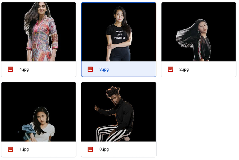
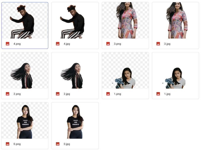
画像フォルダ内のすべての画像が切り抜かれ、保存フォルダに保存されます。

背景は、黒、白、透過から選択できます。

?

---

お仕事のご相談こちらまで
rockyshikoku@gmail.com

Core MLを使ったアプリを作っています。
機械学習関連の情報を発信しています。

Twitter
MLBoysチャンネル
Medium

相棒
note