初めに

• 本記事は、python・機械学習等々を独学している小生の備忘録的な記事になります。
• 「自身が気になったコードを写経しながら勉強していく」という、きわめてシンプルなものになります。
• 建設的なコメントを頂けますと幸いです（気に入ったらLGTM & ストックしてください）。

お題：Classify_images_Using_Python & Machine Learning

今日のお題は、Classify_images_Using_Python & Machine LearningというYoutube上の動画です。犬やら猫らの画像を学習させてそれを判定する、といったものです。

Classify Images Using Python & Machine Learning

分析はyoutubeの動画にある通り、Google Colaboratryを使用しました。

それではやっていきたいと思います。

　Step1: ライブラリのインポート~データの加工

import tensorflow as tf
from tensorflow import keras
from keras.models import Sequential
from keras.layers import Dense, Flatten, Conv2D, MaxPool2D, Dropout
from tensorflow.keras import layers
from keras.utils import to_categorical
import numpy as np
import matplotlib.pyplot as plt
plt.style.use('fivethirtyeight')

次に

1. データの読み込み
2. データ型の確認
3. データシェイプ確認
4. いくつかのデータを確認
5. 画像を一つ出力

までをやっていきます。

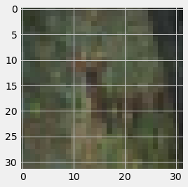
#1
from keras.datasets import cifar10
(x_train, x_test), (y_train, y_test) = cifar10.load_data()

#2
print(type(x_train))
print(type(y_train))
print(type(x_test))
print(type(y_test))

#3
print('x_train shape:', x_train.shape)
print('y_train shape:', y_train.shape)
print('x_test shape:', x_test.shape)
print('y_test shape:', y_test.shape)

#4
index = 10
x_train[index]

#5
img = plt.imshow(x_train[index])

何やら画像が見えてきました。次にこの画像に紐づいているラベルを見ていきます。

print('The image label is:', x_train[index])

これを見ると4というラベルがついていることがわかります。次に開設されてますが、このデータセットは10種類の画像が含まれています。

# Get the image classification
classification = ['airplane', 'automobile', 'bird', 'cat', 'deer', 'dog', 'frog', 'horse', 'ship', 'truck']
# Print the image class
print('The image class is:', classification[y_train[index][0]])

なので、これは「鹿」の画像だそうです（よく画面にめっちゃ寄っても厳しい...）。

次に被説明変数yをone_hot_encodingで、画像ラベルをNeural Networkに入れられる形に0 or 1(正しければ1、そうでなければ0)の数字を当てます。

y_train_one_hot = to_categorical(y_train)
y_test_one_hot = to_categorical(y_test)
print(y_train_one_hot)
print('The one hot label is:', y_train_one_hot[index])

次にデータセットを標準化(0 - 1)にします。

x_train = x_train / 255
x_test = x_test / 255
x_train[index]

これで凡そ加工はおしまいです。次にCNNモデルを組んでいきましょう！

Step2: モデルを構築

model = Sequential()

model.add( Conv2D(32, (5,5), activation='relu', input_shape=(32,32,3)))

model.add(MaxPool2D(pool_size=(2,2)))

model.add( Conv2D(32, (5,5), activation='relu'))

model.add(MaxPool2D(pool_size=(2,2)))

model.add(Flatten())

model.add(Dense(1000, activation='relu'))

model.add(Dropout(0.5))

model.add(Dense(500, activation='relu'))

model.add(Dropout(0.5))

model.add(Dense(250, activation='relu'))

model.add(Dense(10, activation='softmax'))

次にモデルをコンパイルし、学習させていきます。

model.compile(loss= 'categorical_crossentropy',
              optimizer= 'adam',
              metrics= ['accuracy'])


hist = model.fit(x_train, y_train_one_hot,
                 batch_size = 256,
                 epochs = 10,
                 validation_split = 0.2)

出来上がったmodelをtestデータでテストします。

model.evaluate(x_test, y_test_one_hot)[1]
>> 0.6811000108718872

うーん、動画でもそうでしたがあまり良い結果ではないですね。。。

とりあえずmatplotlibで精度と損失誤差を描画しておきます。

# Visualize the model accuracy
plt.plot(hist.history['accuracy'])
plt.plot(hist.history['val_accuracy'])
plt.title('Model accuracy')
plt.ylabel('Accuracy')
plt.xlabel('Epoch')
plt.legend(['Train', 'Val'], loc='upper left')
plt.show()

#Visualize the models loss
plt.plot(hist.history['loss'])
plt.plot(hist.history['val_loss'])
plt.title('Model loss')
plt.ylabel('Loss')
plt.xlabel('Epoch')
plt.legend(['Train', 'Val'], loc='upper right')
plt.show()

最後に適当な画像（今回はネコの画像）を使ってモデルで予測してみます。

# Test the model with an example
from google.colab import files
uploaded = files.upload()

# show the image
new_image = plt.imread('cat-xxxxx.jpeg')
img = plt.imshow(new_image)

# Resize the image
from skimage.transform import resize
resized_image = resize(new_image, (32,32,3))
img = plt.imshow(resized_image)

# Get the models predictions
predictions = model.predict(np.array([resized_image]))
# Show the predictions
predictions

# Sort the predictions from least to greatest
list_index = [0,1,2,3,4,5,6,7,8,9]
x = predictions

for i in range(10):
  for j in range(10):
    if x[0][list_index[i]] > x[0][list_index[j]]:
      temp = list_index[i]
      list_index[i] = list_index[j]
      list_index[j] = temp

# Show the sorted labels in order
print(list_index)

# Print the first 5 predictions
for i in range(5):
  print(classification[list_index[i]], ':', round(predictions[0][list_index[i]] * 100, 2), '%')

結果は、

cat : 51.09 %
dog : 48.73 %
deer : 0.06 %
bird : 0.04 %
frog : 0.04 %

とネコかイヌかほぼ判定できていない結果に（笑）モデルの精度がイマイチ且つ使った画像が良くなかったです。

最後に

今回はtensorflowとkerasを使った画像判定の勉強をしました。もちろん使い物になる精度出ないことは重々承知ですが、足掛かりとしては良かったかなと思います。

引き続きよろしくです。

(これまでの学習)
1. 【1日1写経】Predict employee attrition【Daily_Coding_001】
2. 【1日1写経】Build a Stock Prediction Program【Daily_Coding_002】