- 投稿日:2020-10-13T17:28:25+09:00
アプリでまなぶNN:kerasでテンソルフロープレイグラウンドを理解
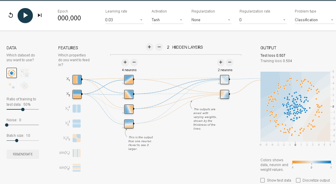
テンソルフロープレイグラウンド(Neural Network Playground)はブラウザー上で動うニューラルネットワークの学習用アプリケーションです。動かすことで簡単に短期間でニューラルネットワークを理解することができます。
これをkerasを用いて理解するのが本記事の目的です。サークル
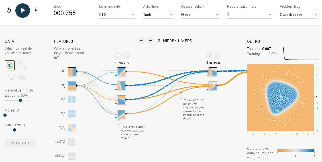
上述の画像はテンソルフロープレイグラウンドの初期画面です。出力データにサークルが選択され、入力データにX1とX2が選ばれています。実行してみます。
これが何を行っているかを正確に理解するために、同じ動きをKerasで実現してみるのも一つの手です。そこでつぎのようなプログラムを作ってみました。
# 初期化
%matplotlib inline
import pandas_datareader.data as web
import matplotlib.pyplot as plt
import numpy as np
import pandas as pd
import datetime

import keras

from keras.models import Sequential
from keras.layers import Dense, Activation

from keras.optimizers import SGD
from keras import models
from keras import layers
from keras import regularizers

from sklearn.metrics import mean_squared_error
from sklearn.model_selection import train_test_split
データの構築
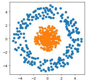
n=250
theta=np.random.uniform(0, 360, n)

x1=np.sin(theta)*np.random.uniform(3,5, n)
x2=np.cos(theta)*np.random.uniform(3,5, n)
y=np.ones(n)

plt.figure(figsize=(4, 4), dpi=50)
plt.scatter(x1,x2)

theta=np.random.uniform(0, 360, n)

x11=np.sin(theta)*np.random.uniform(-0, 2, n)
x22=np.cos(theta)*np.random.uniform(-0,2, n)

yy=np.zeros(n)

plt.scatter(x11,x22)
実行結果
# 訓練データ、テストデータの作成
x1=np.concatenate([x1,x11],axis=0)
x2=np.concatenate([x2,x22],axis=0)
y=np.concatenate([y,yy],axis=0)
X=np.stack([x1,x2],1)#.reshape(-1,2)

X_train, X_test, y_train, y_test = train_test_split(
    X, y, test_size=0.5, random_state=42)
ネットワークの構築と最適化
model = models.Sequential()
model.add(layers.Dense(8, activation='tanh', input_shape=(2,)))
model.add(layers.Dense(8, activation='tanh'))
model.add(layers.Dense(1, activation='sigmoid'))

model.compile(optimizer='rmsprop',
              loss='binary_crossentropy',
              metrics=['accuracy'])
model.fit(
    X_train,
    y_train,
    batch_size=10,
    epochs=500,
    verbose=0)
# 結果の評価 results = model.evaluate(X_train, y_train) results # 8/8 [==============================] - 0s 1ms/step - loss: 3.0139e-05 - accuracy: 1.0000 # [3.0139368391246535e-05, 1.0] results = model.evaluate(X_test, y_test) results # 8/8 [==============================] - 0s 2ms/step - loss: 1.6788e-04 - accuracy: 1.0000 # [0.0001678814151091501, 1.0]どちらの結果も誤差はゼロです。全問正解でした。
参考:
「シミュレーターでまなぶニューラルネットワーク」(アマゾンkindle出版)
「脳・心・人工知能 数理で脳を解き明かす」(ブルーバックス)
「圧縮センシングにもとづくスパースモデリングへのアプローチ」
- 投稿日:2020-10-13T16:46:59+09:00
初めてtensorflowやってみた
タイトル通り初めてtensorflowやってみて環境構築に四苦八苦したので書いてみました。
Qiita初めて書くので説明がうまくないかもですが、よろしくお願いします。構築した環境
私が構築した環境を大雑把に説明します。
- Windows10 Education 2004
- Anaconda3 2020.07 (Python3.83)
- tensorflow-gpu 2.30
- CPU : Ryzen7 1700
- GPU : GTX 1060 6GB
まずPythonの環境構築
Anaconda3 から下にあるGraphical Installerをダウンロード、OS,bitは環境に合わせて選択してください。
インストーラのガイドに従ってインストール、チェックなどはそのままでも大丈夫です。
インストールが終わったら、Anaconda prompt を起動
tensorflow-gpu 2.30 をインストールするために tensorflow pipガイド の下のリストから自分の環境に合わせたものをダウンロード
tensorflowのパッケージファイルをダウンロードしたら、
pip install --upgrade [ダウンロードしたファイル]とAnaconda prompt に入力してインストールNvidia GPU環境の構築
ここからはNvidia GPUを利用したい人向けです。
参考にさせていただいた記事のよるとtensorflow 2.3 はCUDA 10.1,cuDNN 7.6で動作するようです。私の環境でもこの組み合わせで動作しました。
tensorflow のバージョンに合わせてCUDA, cuDNN を導入してください。またtensorflowでGPUを使用するためにはメモリ使用量の設定をしないといけないようです。
そのために下記のコードをコードの先頭に記述します。pythonphysical_devices = tf.config.list_physical_devices('GPU') if len(physical_devices) > 0: for device in physical_devices: tf.config.experimental.set_memory_growth(device, True) print('{} memory growth: {}'.format(device, tf.config.experimental.get_memory_growth(device))) else: print("Not enough GPU hardware devices available")コードの記述はtensorflowのバージョンによって異なりますので、私が参考にさせていただいた記事をご参照ください。
tensorflowを試してみる
tensorflow のチュートリアルにあるニューラルネットワークを使った画像の分類をやってみます。
GPUで処理をするために先程のコードを追加しています。newralnet_demo.py# TensorFlow と tf.keras のインポート import tensorflow as tf from tensorflow import keras # ヘルパーライブラリのインポート import numpy as np import matplotlib.pyplot as plt # import os # os.environ['CUDA_VISIBLE_DEVICES'] = '-1' # print(tf.__version__) # GPU_settings physical_devices = tf.config.list_physical_devices('GPU') if len(physical_devices) > 0: for device in physical_devices: tf.config.experimental.set_memory_growth(device, True) print('{} memory growth: {}'.format( device, tf.config.experimental.get_memory_growth(device))) else: print("Not enough GPU hardware devices available") fashion_mnist = keras.datasets.fashion_mnist (train_images, train_labels), (test_images, test_labels) = fashion_mnist.load_data() class_names = ['T-shirt/top', 'Trouser', 'Pullover', 'Dress', 'Coat', 'Sandal', 'Shirt', 'Sneaker', 'Bag', 'Ankle boot'] train_images.shape len(train_labels) train_labels test_images.shape len(test_labels) plt.figure() plt.imshow(train_images[0]) plt.colorbar() plt.grid(False) plt.show() train_images = train_images / 255.0 test_images = test_images / 255.0 plt.figure(figsize=(10, 10)) for i in range(25): plt.subplot(5, 5, i+1) plt.xticks([]) plt.yticks([]) plt.grid(False) plt.imshow(train_images[i], cmap=plt.cm.binary) plt.xlabel(class_names[train_labels[i]]) plt.show() model = keras.Sequential([ keras.layers.Flatten(input_shape=(28, 28)), keras.layers.Dense(128, activation='relu'), keras.layers.Dense(10, activation='softmax') ]) model.compile(optimizer='adam', loss='sparse_categorical_crossentropy', metrics=['accuracy']) model.fit(train_images, train_labels, epochs=5) test_loss, test_acc = model.evaluate(test_images, test_labels, verbose=2) print('\nTest accuracy:', test_acc) predictions = model.predict(test_images) predictions[0] np.argmax(predictions[0]) test_labels[0] def plot_image(i, predictions_array, true_label, img): predictions_array, true_label, img = predictions_array[i], true_label[i], img[i] plt.grid(False) plt.xticks([]) plt.yticks([]) plt.imshow(img, cmap=plt.cm.binary) predicted_label = np.argmax(predictions_array) if predicted_label == true_label: color = 'blue' else: color = 'red' plt.xlabel("{} {:2.0f}% ({})".format(class_names[predicted_label], 100*np.max(predictions_array), class_names[true_label]), color=color) def plot_value_array(i, predictions_array, true_label): predictions_array, true_label = predictions_array[i], true_label[i] plt.grid(False) plt.xticks([]) plt.yticks([]) thisplot = plt.bar(range(10), predictions_array, color="#777777") plt.ylim([0, 1]) predicted_label = np.argmax(predictions_array) thisplot[predicted_label].set_color('red') thisplot[true_label].set_color('blue') i = 0 plt.figure(figsize=(6, 3)) plt.subplot(1, 2, 1) plot_image(i, predictions, test_labels, test_images) plt.subplot(1, 2, 2) plot_value_array(i, predictions, test_labels) plt.show() i = 12 plt.figure(figsize=(6, 3)) plt.subplot(1, 2, 1) plot_image(i, predictions, test_labels, test_images) plt.subplot(1, 2, 2) plot_value_array(i, predictions, test_labels) plt.show() # X個のテスト画像、予測されたラベル、正解ラベルを表示します。 # 正しい予測は青で、間違った予測は赤で表示しています。 num_rows = 5 num_cols = 3 num_images = num_rows*num_cols plt.figure(figsize=(2*2*num_cols, 2*num_rows)) for i in range(num_images): plt.subplot(num_rows, 2*num_cols, 2*i+1) plot_image(i, predictions, test_labels, test_images) plt.subplot(num_rows, 2*num_cols, 2*i+2) plot_value_array(i, predictions, test_labels) plt.show() # テスト用データセットから画像を1枚取り出す img = test_images[0] print(img.shape) # 画像を1枚だけのバッチのメンバーにする img = (np.expand_dims(img, 0)) print(img.shape) predictions_single = model.predict(img) print(predictions_single) plot_value_array(0, predictions_single, test_labels) _ = plt.xticks(range(10), class_names, rotation=45) np.argmax(predictions_single[0])処理がうまく行けば画像が分類されて一覧で表示されます。
参考にしたサイト
金子邦彦研究室様のwebサイトをかなり参考にさせていただきました。
とても参考になりました。ありがとうございます。


