- 投稿日:2019-02-03T19:33:47+09:00
高精度な物体検出器SNIPER+MXNetの環境構築
はじめに
高精度な物体検出器のSoTA1の1つとしてSNIPERがあります。
SNIPER: Efficient Multi-Scale Training [Bharat Singh+, NeurIPS2018] https://arxiv.org/abs/1805.09300コードも公開されている( https://github.com/mahyarnajibi/SNIPER )のですが、フレームワークがMXNetな上、ビルド済みMXNetが使えず環境構築に難儀します。そこで本記事では、github上の最新のMXNetとSNIPERをマージして使用する際の環境構築手順をまとめます。不正確な部分もあるかと思いますが、一から調べて環境構築するよりかは辛みが軽減されると思いますのでご容赦下さい。
- 注意事項:
Prerequisites
MXNetに必要なライブラリを事前にインストールします。環境によって、またMXNetのビルド設定によって不要なものもあるため、以下は一例です。condaは必須ではないですが、Python 2 と 3 を切り替えやすくする手段は用意した方が良いと思います。
# Install CUDA 10.0 to Ubuntu 18.04
wget https://developer.download.nvidia.com/compute/cuda/repos/ubuntu1804/x86_64/cuda-repo-ubuntu1804_10.0.130-1_amd64.deb
sudo dpkg -i cuda-repo-ubuntu1804_10.0.130-1_amd64.deb
sudo apt-key adv --fetch-keys https://developer.download.nvidia.com/compute/cuda/repos/ubuntu1804/x86_64/7fa2af80.pub
sudo apt-get update
sudo apt-get install -y cuda
rm cuda-repo-ubuntu1804_10.0.130-1_amd64.deb
echo 'export PATH=/usr/local/cuda/bin:${PATH}' >> ~/.bashrc
echo 'export LD_LIBRARY_PATH=/usr/local/cuda/lib64:${LD_LIBRARY_PATH}' >> ~/.bashrc
source ~/.bashrc

# Install cuDNN
wget http://developer.download.nvidia.com/compute/redist/cudnn/v7.4.1/cudnn-10.0-linux-x64-v7.4.1.5.tgz
tar -xf cudnn-10.0-linux-x64-v7.4.1.5.tgz
sudo cp -a cuda/lib64/* /usr/local/cuda/lib64/
sudo cp -a cuda/include/* /usr/local/cuda/include/
sudo ldconfig
sudo rm -r cuda cudnn-10.0-linux-x64-v7.4.1.5.tgz

# Install mkl
# TODO: try to run https://github.com/apache/incubator-mxnet/blob/master/ci/docker/install/ubuntu_mkl.sh
wget https://apt.repos.intel.com/intel-gpg-keys/GPG-PUB-KEY-INTEL-SW-PRODUCTS-2019.PUB
sudo apt-key add GPG-PUB-KEY-INTEL-SW-PRODUCTS-2019.PUB
sudo wget https://apt.repos.intel.com/setup/intelproducts.list -O /etc/apt/sources.list.d/intelproducts.list
sudo apt-get update
sudo apt-get install -y intel-mkl-2019.1-053
rm GPG-PUB-KEY-INTEL-SW-PRODUCTS-2019.PUB

# Install NCCL
# See https://qiita.com/pst-ic/items/e01033dee4d389df3a5e
# TODO: Validating NCCL https://mxnet.incubator.apache.org/versions/master/install/build_from_source.html#validating-nccl
git clone https://github.com/NVIDIA/nccl.git
cd nccl
make -j
sudo mkdir /usr/local/nccl
sudo make PREFIX=/usr/local/nccl install -j
cd ../
sudo rm -r nccl
echo 'export NCCL_ROOT="/usr/local/nccl"' >> ~/.bashrc
echo 'export CPATH="$NCCL_ROOT/include:$CPATH"' >> ~/.bashrc
echo 'export LD_LIBRARY_PATH="$NCCL_ROOT/lib/:$LD_LIBRARY_PATH"' >> ~/.bashrc
echo 'export LIBRARY_PATH="$NCCL_ROOT/lib/:$LIBRARY_PATH"' >> ~/.bashrc
source ~/.bashrc

# Install miniconda
wget https://repo.anaconda.com/miniconda/Miniconda2-latest-Linux-x86_64.sh
bash Miniconda2-latest-Linux-x86_64.sh -b
echo 'export PATH="$HOME/miniconda2/bin:$PATH"' >> ~/.bashrc
source ~/.bashrc
rm Miniconda2-latest-Linux-x86_64.sh

sudo reboot
Install MXNet
MXNetの最新版にSNIPER用のoperatorをマージした上でMXNetをビルドします。古き良きCaffeの時代を彷彿とさせますね。ビルドに時間がかかる時はmake coffeeしながら気長に待ちましょう。
# merge incubator-mxnet and SNIPER-mxnet
mkdir work
cd work
git clone --recursive https://github.com/apache/incubator-mxnet.git
git clone --recursive https://github.com/mahyarnajibi/SNIPER.git
# remove conflicting files. See https://github.com/mahyarnajibi/SNIPER-mxnet/commit/d640d3e92fb54daaf2eb427f3fcb5683ab60a005
rm incubator-mxnet/src/operator/contrib/multi_proposal* incubator-mxnet/src/operator/contrib/proposal*
# copy operators for SNIPER. See https://github.com/mahyarnajibi/SNIPER/issues/9
cp SNIPER/SNIPER-mxnet/src/operator/multi_proposal* incubator-mxnet/src/operator/

# Build MXNet from Source
# See https://mxnet.incubator.apache.org/versions/master/install/ubuntu_setup.html
#     https://mxnet.incubator.apache.org/versions/master/install/build_from_source.html
#     https://github.com/apache/incubator-mxnet/blob/master/ci/docker/install/ubuntu_python.sh
sudo bash incubator-mxnet/ci/docker/install/ubuntu_core.sh
conda install numpy=1.15.2
pip install nose cpplint==1.3.0 pylint==1.9.3 nose-timer 'requests<2.19.0,>=2.18.4' h5py==2.8.0rc1 scipy==1.0.1 boto3

cd incubator-mxnet/
make -j $(nproc) USE_OPENCV=1 USE_LAPACK=1 USE_MKLDNN=1 USE_BLAS=mkl USE_CUDA=1 USE_CUDA_PATH=/usr/local/cuda USE_CUDNN=1 USE_NCCL=1 USE_NCCL_PATH=/usr/local/nccl

# https://mxnet.incubator.apache.org/install/ubuntu_setup.html
cd python
pip install -e .

# change path of MXNet in SNIPER/init.py
cd
cd work/SNIPER/
echo "import sys" > init.py
echo "sys.path.insert(0, 'lib')" >> init.py
echo "sys.path.insert(0, '../incubator-mxnet/python')" >> init.py
Install SNIPER
ここまで来れば https://github.com/mahyarnajibi/SNIPER に従って動かせるかと思います。
pip install -r requirements.txt
bash scripts/compile.sh

echo 'export LD_LIBRARY_PATH="$HOME/work/incubator-mxnet/lib:${LD_LIBRARY_PATH}"' >> ~/.bashrc
source ~/.bashrc

# Running the demo
bash scripts/download_sniper_detector.sh
python demo.py
お疲れ様でした。
様々なテクニックが併用されているにも関わらず、単にベンチマークでトップ精度を達成しているものがstate-of-the-artと呼ばれ崇め奉られることの是非はさておき、ベースとして用いる実装の候補としては良いでしょう。 ↩
Deformable Convolutional Networksのコードがベースとなっているためかと思います。 ↩
GCE の ubuntu-1804-bionic-v20181222 で検証しています。なお、colab上でもSNIPERの訓練・評価は可能です(特定のバージョンのCUDAが最初から入っていることが、本記事の内容との主な違いです)。 ↩
- 投稿日:2019-02-03T02:15:56+09:00
新PCが届いたので動作確認がてら、畳み込みニューラルネットワークで画像を分類
前置き
久しぶりになってしまいました。
GPU搭載PCを購入して届いたので、GPGPUのテストのために、MNISTを解く畳み込みニューラルネットワーク(Convolutional Neural Network)を組んだので、記事にしておきます。
MNISTなので、入力は(n, 28, 28, 1)で出力はOne-Hot行列で10次元(n, 10)です。
この間を畳み込みやプーリングで局所的な特徴を捉えたり、情報圧縮を図って分類精度を確保するのがCNNです。以前、単層パーセプトロンで同じMNISTに取り組みましたが、あれは画像を縦横二次元の画像として扱えていなかったり、非線形性を持てない表現力で精度の限界がすぐにやってきてしまいますが、こちらの精度はあんな物ではありません。
とは言え、GPUによるアクセラレーションができるようになったことを確認できたらいいので、あんまり突き詰めるつもりはありません。環境
PCやライブラリの環境は下記を構築しました。
バージョンの互換性合わせとかで半日ぐらいかかってしまいました。Windows 10 CUDA Toolkit 9.0 cudnn 7.3.1.20 Python 3.6.1 Keras 2.2.4 (Tensorflow 1.12.0 backend)ソースコード全文
また先にソースコード全文です。
データ用意、モデル作って、学習させて、最後に評価。今回は間違えたデータの可視化までしました。
間違えたデータの共通点からモデルの改善点を見つけましょう。# -*- coding: utf-8 -*- import numpy as np import pandas as pd import matplotlib.pyplot as plt import keras.backend as K from keras.datasets import mnist from keras.models import Sequential from keras.layers import Conv2D, MaxPool2D, Activation, Flatten, Dense, BatchNormalization from keras.utils import to_categorical from sklearn.metrics import classification_report, confusion_matrix def conv_block(instance, f, fsize, pool): instance.add(Conv2D(f, fsize)) instance.add(BatchNormalization()) instance.add(Activation('relu')) if pool != None: instance.add(MaxPool2D(pool)) def cnn_model(): ret = Sequential() ret.add(Conv2D(32, (5, 5), input_shape=(size_h, size_w, size_c))) ret.add(BatchNormalization()) ret.add(Activation('relu')) for f, p in zip([32, 64, 64, 128, 128], [(2, 2), None, (2, 2), None, (2, 2)]): conv_block(ret, f, (2, 2), p) ret.add(Flatten()) ret.add(Dense(64)) ret.add(Activation('relu')) ret.add(Dense(10)) ret.add(Activation('softmax')) ret.compile(optimizer='adam', loss='categorical_crossentropy', metrics=['acc']) print(ret.summary()) return ret if __name__ == '__main__': size_h, size_w, size_c = 28, 28, 1 (x_train, y_train), (x_test, y_test) = mnist.load_data() x_train = x_train.reshape(-1, size_h, size_w, size_c) / 255. x_test = x_test.reshape(-1, size_h, size_w, size_c) / 255. y_train_cate = to_categorical(y_train) y_test_cate = to_categorical(y_test) K.clear_session() dnn = cnn_model() e_ = 10 b_ = 1024 dnn.fit(x_train, y_train_cate, epochs=e_, batch_size=b_, validation_data=(x_test, y_test_cate)) p_train = dnn.predict_classes(x_train) p_test = dnn.predict_classes(x_test) cm_train = pd.DataFrame(confusion_matrix(y_train, p_train), columns=np.arange(0, 10)) cm_train.index = np.arange(0, 10) cm_test = pd.DataFrame(confusion_matrix(y_test, p_test), columns=np.arange(0, 10)) cm_test.index = np.arange(0, 10) print('Train Data Confusion Matrix') print(cm_train) print('Classification Report') print(classification_report(y_train, p_train)) print('') print('Test Data') print(cm_test) print('Classification Report') print(classification_report(y_test, p_test)) e_train = x_train[y_train != p_train] tl_train = y_train[y_train != p_train] pl_train = p_train[y_train != p_train] e_test = x_test[y_test != p_test] tl_test = y_test[y_test != p_test] pl_test = p_test[y_test != p_test] pcnt = 1 fig = plt.figure() if len(e_train) > 0: for i in range(len(e_train[:16])): fig.add_subplot(4, 8, pcnt) plt.imshow(e_train[i].reshape(size_h, size_w), cmap='binary') plt.xticks([]) plt.yticks([]) plt.title('Train Data\nTrue:' + str(tl_train[i]) + ';Predict:' + str(pl_train[i])) pcnt += 1 if len(e_test) > 0: for i in range(len(e_test[:32-pcnt+1])): fig.add_subplot(4, 8, pcnt) plt.imshow(e_test[i].reshape(size_h, size_w), cmap='binary') plt.xticks([]) plt.yticks([]) plt.title('Test Data\nTrue:' + str(tl_test[i]) + ';Predict:' + str(pl_test[i])) pcnt += 1解説
ライブラリのインポート
import numpy as np import pandas as pd import matplotlib.pyplot as plt import keras.backend as K from keras.datasets import mnist from keras.models import Sequential from keras.layers import Conv2D, MaxPool2D, Activation, Flatten, Dense, BatchNormalization from keras.utils import to_categorical from sklearn.metrics import classification_report, confusion_matrixConv2Dが畳み込み層、MaxPool2Dが最大プーリング層です。
他や詳しいことはKerasのリファレンスを読むのがよいと思います。
BatchNormalizationは入力値を平均0標準偏差1になるように正規化します。
これを全結合層や畳み込み層の後に入れることで、精度向上や収束の高速化が繋がります(当然、絶対にではない)。
分類問題としてのRecallやPrecisionなどの精度指標を見ようと思いますので、
scikit-learnのclassification_reportとconfusion_matrixもインポートします。モデル構築
def conv_block(instance, f, fsize, pool):
    instance.add(Conv2D(f, fsize))
    instance.add(BatchNormalization())
    instance.add(Activation('relu'))
    if pool != None:
        instance.add(MaxPool2D(pool))

def cnn_model():
    ret = Sequential()

    ret.add(Conv2D(32, (5, 5), input_shape=(size_h, size_w, size_c)))
    ret.add(BatchNormalization())
    ret.add(Activation('relu'))

    for f, p in zip([32, 64, 64, 128, 128], [(2, 2), None, (2, 2), None, (2, 2)]):
        conv_block(ret, f, (2, 2), p)

    ret.add(Flatten())
    ret.add(Dense(64))
    ret.add(Activation('relu'))

    ret.add(Dense(10))
    ret.add(Activation('softmax'))

    ret.compile(optimizer='adam', loss='categorical_crossentropy', metrics=['acc'])
    print(ret.summary())

    return ret
モデルはこんな感じですが、ループで構築しちゃったりしてるので、print(ret.summary())の標準出力の方がデータがどのように変形していくのかわかりやすいので、そちらを載せておきます。
_________________________________________________________________
Layer (type)                 Output Shape              Param #
=================================================================
conv2d_1 (Conv2D)            (None, 24, 24, 32)        832
_________________________________________________________________
batch_normalization_1 (Batch (None, 24, 24, 32)        128
_________________________________________________________________
activation_1 (Activation)    (None, 24, 24, 32)        0
_________________________________________________________________
conv2d_2 (Conv2D)            (None, 23, 23, 32)        4128
_________________________________________________________________
batch_normalization_2 (Batch (None, 23, 23, 32)        128
_________________________________________________________________
activation_2 (Activation)    (None, 23, 23, 32)        0
_________________________________________________________________
max_pooling2d_1 (MaxPooling2 (None, 11, 11, 32)        0
_________________________________________________________________
conv2d_3 (Conv2D)            (None, 10, 10, 64)        8256
_________________________________________________________________
batch_normalization_3 (Batch (None, 10, 10, 64)        256
_________________________________________________________________
activation_3 (Activation)    (None, 10, 10, 64)        0
_________________________________________________________________
conv2d_4 (Conv2D)            (None, 9, 9, 64)          16448
_________________________________________________________________
batch_normalization_4 (Batch (None, 9, 9, 64)          256
_________________________________________________________________
activation_4 (Activation)    (None, 9, 9, 64)          0
_________________________________________________________________
max_pooling2d_2 (MaxPooling2 (None, 4, 4, 64)          0
_________________________________________________________________
conv2d_5 (Conv2D)            (None, 3, 3, 128)         32896
_________________________________________________________________
batch_normalization_5 (Batch (None, 3, 3, 128)         512
_________________________________________________________________
activation_5 (Activation)    (None, 3, 3, 128)         0
_________________________________________________________________
conv2d_6 (Conv2D)            (None, 2, 2, 128)         65664
_________________________________________________________________
batch_normalization_6 (Batch (None, 2, 2, 128)         512
_________________________________________________________________
activation_6 (Activation)    (None, 2, 2, 128)         0
_________________________________________________________________
max_pooling2d_3 (MaxPooling2 (None, 1, 1, 128)         0
_________________________________________________________________
flatten_1 (Flatten)          (None, 128)               0
_________________________________________________________________
dense_1 (Dense)              (None, 64)                8256
_________________________________________________________________
activation_7 (Activation)    (None, 64)                0
_________________________________________________________________
dense_2 (Dense)              (None, 10)                650
_________________________________________________________________
activation_8 (Activation)    (None, 10)                0
=================================================================
Total params: 138,922
Trainable params: 138,026
Non-trainable params: 896
_________________________________________________________________
None
データの用意
if __name__ == '__main__':
    size_h, size_w, size_c = 28, 28, 1
    (x_train, y_train), (x_test, y_test) = mnist.load_data()
    x_train = x_train.reshape(-1, size_h, size_w, size_c) / 255.
    x_test = x_test.reshape(-1, size_h, size_w, size_c) / 255.
    y_train_cate = to_categorical(y_train)
    y_test_cate = to_categorical(y_test)
ここからmainです。
といってもここはデータの用意だけです。
MNISTの訓練用6万件のデータと検証用1万件データを取り込みます。
Kerasの畳み込み層は色のチャンネルが必須とされているので、グレースケール画像でも最後に1というチャンネルが必要ですので、これをNumpyのreshapeで付け加えます。
目的変数のデータはOne-Hot行列に変換しますが、後で使うscikit-learnの方はOne-Hot行列を想定していないので、One-Hot行列の方は別変数に確保しておきます。学習
    K.clear_session()
    dnn = cnn_model()
    e_ = 10
    b_ = 1024
    dnn.fit(x_train, y_train_cate, epochs=e_, batch_size=b_, validation_data=(x_test, y_test_cate))
ここは特に解説はないです。
・・・しいて言うとMNISTは似たようなデータが多いので、バッチサイズは大きめに取った方が良いです。
学習中の標準出力の最初の方と最後の方を抜粋しておきます。Train on 60000 samples, validate on 10000 samples Epoch 1/10 60000/60000 [==============================] - 7s 124us/step - loss: 0.3911 - acc: 0.8879 - val_loss: 0.1085 - val_acc: 0.9674 Epoch 2/10 60000/60000 [==============================] - 6s 105us/step - loss: 0.0589 - acc: 0.9832 - val_loss: 0.0657 - val_acc: 0.9814 Epoch 3/10 60000/60000 [==============================] - 6s 105us/step - loss: 0.0330 - acc: 0.9912 - val_loss: 0.0556 - val_acc: 0.9829 -------------------------------- Epoch 8/10 60000/60000 [==============================] - 6s 104us/step - loss: 0.0025 - acc: 0.9999 - val_loss: 0.0310 - val_acc: 0.9901 Epoch 9/10 60000/60000 [==============================] - 6s 105us/step - loss: 0.0015 - acc: 1.0000 - val_loss: 0.0292 - val_acc: 0.9911 Epoch 10/10 60000/60000 [==============================] - 6s 105us/step - loss: 0.0011 - acc: 1.0000 - val_loss: 0.0288 - val_acc: 0.9922評価
p_train = dnn.predict_classes(x_train)
    p_test = dnn.predict_classes(x_test)
    cm_train = pd.DataFrame(confusion_matrix(y_train, p_train), columns=np.arange(0, 10))
    cm_train.index = np.arange(0, 10)
    cm_test = pd.DataFrame(confusion_matrix(y_test, p_test), columns=np.arange(0, 10))
    cm_test.index = np.arange(0, 10)
    print('Train Data Confusion Matrix')
    print(cm_train)
    print('Classification Report')
    print(classification_report(y_train, p_train))
    print('')
    print('Test Data')
    print(cm_test)
    print('Classification Report')
    print(classification_report(y_test, p_test))

    e_train = x_train[y_train != p_train]
    tl_train = y_train[y_train != p_train]
    pl_train = p_train[y_train != p_train]
    e_test = x_test[y_test != p_test]
    tl_test = y_test[y_test != p_test]
    pl_test = p_test[y_test != p_test]

    pcnt = 1
    fig = plt.figure()
    if len(e_train) > 0:
        for i in range(len(e_train[:16])):
            fig.add_subplot(4, 8, pcnt)
            plt.imshow(e_train[i].reshape(size_h, size_w), cmap='binary')
            plt.xticks([])
            plt.yticks([])
            plt.title('Train Data' + str(i+1) + '\nTrue:' + str(tl_train[i]) + ';Predict:' + str(pl_train[i]))
            pcnt += 1
    if len(e_test) > 0:
        for i in range(len(e_test[:32-pcnt+1])):
            fig.add_subplot(4, 8, pcnt)
            plt.imshow(e_test[i].reshape(size_h, size_w), cmap='binary')
            plt.xticks([])
            plt.yticks([])
            plt.title('Test Data' + str(i+1) + '\nTrue:' + str(tl_test[i]) + ';Predict:' + str(pl_test[i]))
            pcnt += 1
ここは評価をしやすいようにデータを可視化したり行列化したりしています。
scikit-learnのclassification_reportとconfusion_matrixはこんな感じです。Train Data Confusion Matrix 0 1 2 3 4 5 6 7 8 9 0 5923 0 0 0 0 0 0 0 0 0 1 0 6742 0 0 0 0 0 0 0 0 2 0 0 5958 0 0 0 0 0 0 0 3 0 0 0 6131 0 0 0 0 0 0 4 0 0 0 0 5842 0 0 0 0 0 5 0 0 0 0 0 5421 0 0 0 0 6 0 0 0 0 0 0 5918 0 0 0 7 0 0 0 0 0 0 0 6265 0 0 8 0 0 0 0 0 0 0 0 5851 0 9 0 0 0 0 0 0 0 0 0 5949 Classification Report precision recall f1-score support 0 1.00 1.00 1.00 5923 1 1.00 1.00 1.00 6742 2 1.00 1.00 1.00 5958 3 1.00 1.00 1.00 6131 4 1.00 1.00 1.00 5842 5 1.00 1.00 1.00 5421 6 1.00 1.00 1.00 5918 7 1.00 1.00 1.00 6265 8 1.00 1.00 1.00 5851 9 1.00 1.00 1.00 5949 micro avg 1.00 1.00 1.00 60000 macro avg 1.00 1.00 1.00 60000 weighted avg 1.00 1.00 1.00 60000 Test Data 0 1 2 3 4 5 6 7 8 9 0 974 0 1 0 0 1 2 1 0 1 1 0 1131 1 2 0 0 0 1 0 0 2 1 1 1026 0 0 0 0 4 0 0 3 0 0 1 1003 0 5 0 0 1 0 4 0 0 0 0 978 0 1 0 0 3 5 2 0 0 4 0 881 3 1 0 1 6 2 3 0 0 2 3 948 0 0 0 7 0 5 3 1 0 0 0 1018 1 0 8 1 0 2 1 1 1 0 0 966 2 9 2 0 0 1 6 1 0 2 0 997 Classification Report precision recall f1-score support 0 0.99 0.99 0.99 980 1 0.99 1.00 0.99 1135 2 0.99 0.99 0.99 1032 3 0.99 0.99 0.99 1010 4 0.99 1.00 0.99 982 5 0.99 0.99 0.99 892 6 0.99 0.99 0.99 958 7 0.99 0.99 0.99 1028 8 1.00 0.99 0.99 974 9 0.99 0.99 0.99 1009 micro avg 0.99 0.99 0.99 10000 macro avg 0.99 0.99 0.99 10000 weighted avg 0.99 0.99 0.99 10000訓練データは100%正解です。
検証データはちょっと間違っています。
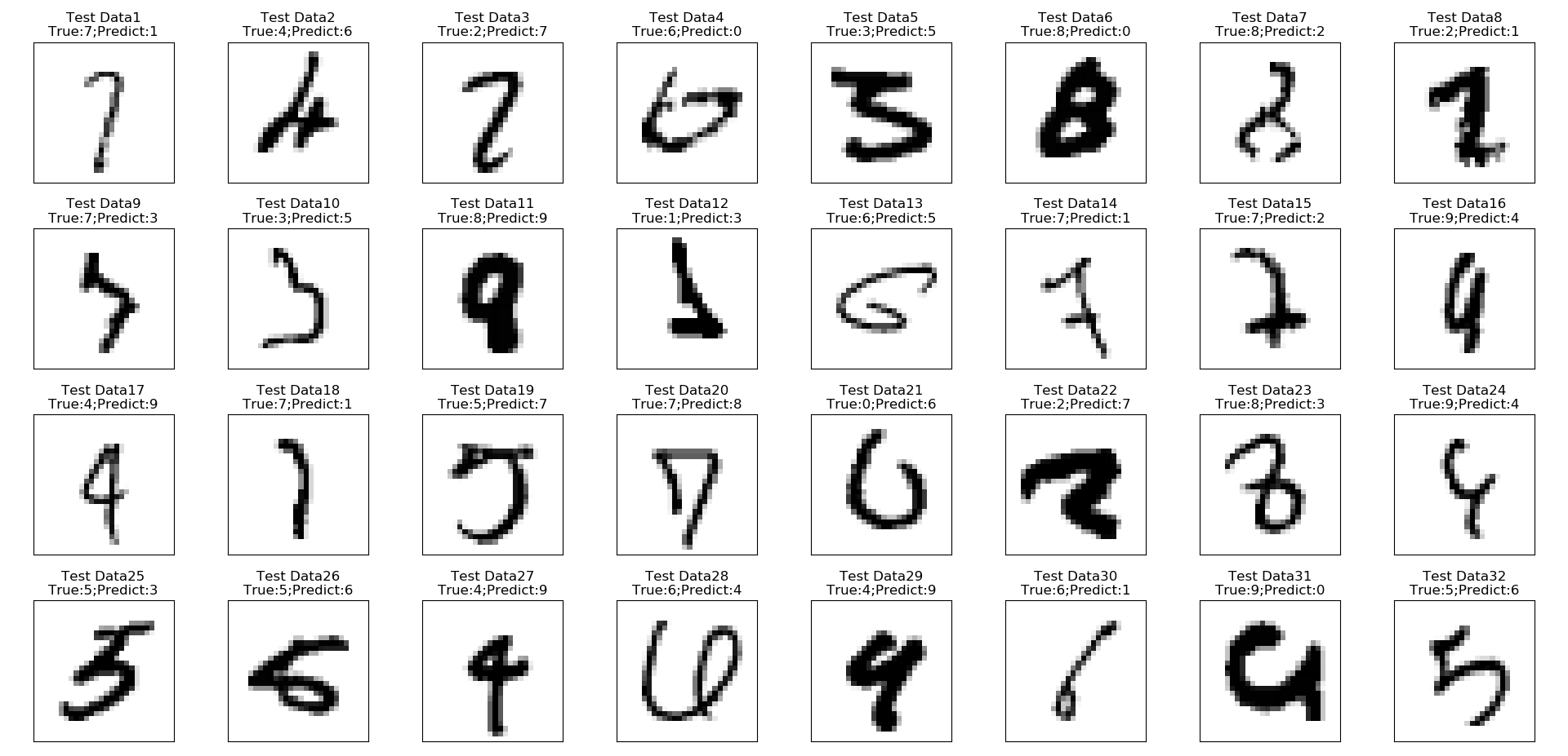
間違ってしまったデータの可視化をmatplotlibで可視化しています。
結果はこちら。Trueが正解ラベル、Predictが予測ラベルです。
訓練データも間違っていたら出すようにしたんですが、ひとつも間違えていないので、全部検証データです。
MNISTのデータはトリッキーなやつが含まれていて、ここでもそれがよくわかります。
例えば1番と18番の7は1と、11番の8は9と、21番の0は6、28番の6は4と間違えてますが、見た目上無理も無いです。
逆にこれは正解してほしいというような6番みたいなのもあります。
ここでPrecisionやRecall等と見比べていくと、8という数字の覚え方が良さそうか良くなさそうか判断してモデルのチューニングをしていきます。訓練データが100%な点からも過学習しているかもしれませんね。今回の目的上、これ以上は進めません。
GPUアクセラレーションできたのか?
できました。
いつもSpyderを標準のIDEにして、IPythonから実行させていますが、これでTensorflowをバックエンドにKerasを使うと最初にGPUのメモリを取れるだけ取ってあとはずっと保持しちゃいます。
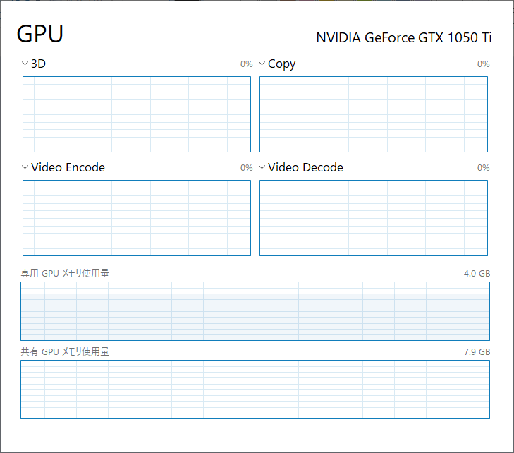
この事から、WindowsのタスクマネージャーからGPUパフォーマンスを見ると・・・
こんな感じに学習終了後も専用GPU使用料が張り付いています。
どのプロセスに取られているかは、同じくタスクマネージャーからプロセス一覧を見ても分かりますが、コマンドプロンプトでnvidia-smiコマンドがオススメです。+-----------------------------------------------------------------------------+ | NVIDIA-SMI 417.71 Driver Version: 417.71 CUDA Version: 10.0 | |-------------------------------+----------------------+----------------------+ | GPU Name TCC/WDDM | Bus-Id Disp.A | Volatile Uncorr. ECC | | Fan Temp Perf Pwr:Usage/Cap| Memory-Usage | GPU-Util Compute M. | |===============================+======================+======================| | 0 GeForce GTX 105... WDDM | 00000000:01:00.0 Off | N/A | | N/A 36C P8 N/A / N/A | 3351MiB / 4096MiB | 0% Default | +-------------------------------+----------------------+----------------------+ +-----------------------------------------------------------------------------+ | Processes: GPU Memory | | GPU PID Type Process name Usage | |=============================================================================| | 0 9024 C C:\ProgramData\Anaconda3\pythonw.exe N/A | +-----------------------------------------------------------------------------+下方のProcessesの所を見るとPythonだと分かります。
他にもGPUを使っているプロセスがあれば、一緒に表示されます。なぜか、右上のCUDA Versionが10.0になってます・・・
確かに最初10.0をインストールしてしまって、Tensorflowがアウトで9.0に落としたんですが・・・
ついでなので、CUDAのバージョンとか見ておきましょう。
CUDAのバージョンを確認するにはnvcc -Vと実行すると見れます。nvcc: NVIDIA (R) Cuda compiler driver Copyright (c) 2005-2017 NVIDIA Corporation Built on Fri_Sep__1_21:08:32_Central_Daylight_Time_2017 Cuda compilation tools, release 9.0, V9.0.176やっぱり9.0じゃないか・・・
ちなみにcudnnの方のバージョンは、cudnnがただのソースコードなので、ソースを見るしかないです。あと、nvidia-smiは一回打つと一回出るだけなので、繰り返させるためには
nvidia-smi -l 1-lオプションの後に何秒おきに繰り返すか設定できます。
Ctrl+Cとかで割込み終了させます。最後に
長くなってしまったので、今回はこの辺にしておこうと思います。
次からソースコードの解説の仕方をちょっと変えないと、毎回長くなってしまいます・・・・
- 投稿日:2019-02-03T01:24:10+09:00
とてもシンプルなAdamを実装する(ベクトル)
ディープラーニングでよく使用されるソルバー、Adam (Kingma, Ba, 2015)を理解するためにpythonでシンプルな実装を行った。
以前、パラメータをスカラー$\theta$として同様の記事を書いたが(とてもシンプルなAdamを実装する(スカラー))、今回はパラメータを2次元のベクトル$\vec{\theta} = (\theta_1, \theta_2) $とした。
モデルは$y=\theta_1 x_1 + \theta_2 x_2$、誤差関数は二乗誤差を使用した。アルゴリズム
この節はスカラー版の記事と同じものを再掲した。
Adamの理論的な面について筆者は別に記事を書いている(俺はまだ本当のAdamを理解していない)。
Adamは生の勾配ではなく、勾配の平均と(中心化前の)分散を使って、パラメータの更新幅が大きくなりすぎないように調節していることが特徴だった。また、この平均と分散を0にバイアスさせない目的で定数$\beta_1,\beta_2$による補正を行っている。Adamのアルゴリズムを再掲する。
アルゴリズム1
$g_t^2$は要素ごとの2乗$g_t \odot g_t $を表す。
ベクトル上のすべての操作は要素ごとに行う。
$\beta_1^t, \beta_2^t$は$\beta_1, \beta_2$の$t$乗のこと。
Require:$\quad \alpha \quad$ ステップサイズ
Require:$\quad \beta_1, \beta_2 \in [0,1) \quad$モーメント推定に使う指数減衰率
Require:$\quad f(\theta) \quad$ パラメターを$\theta$とする確率的目的関数
Require:$\quad \theta_0 \quad$ 初期パラメータベクトル
$\quad m_0 \leftarrow 0 \quad$(最初の一次モーメントベクトル)
$\quad v_0 \leftarrow 0 \quad$(最初の二次モーメントベクトル)
$\quad t \leftarrow 0 \quad$(タイムステップ初期化)
$\quad$ while $\;\theta_t$が収束していない do
$\qquad t \leftarrow t+1$
$\qquad g_t \leftarrow \nabla_\theta f_t (\theta_{t-1}) \quad$ 目的関数の時刻tでの勾配
$\qquad m_t \leftarrow \beta_1 \cdot m_{t-1} +(1-\beta_1) \cdot g_t \quad$ 一次のモーメントを更新(バイアスあり)
$\qquad v_t \leftarrow \beta_2 \cdot v_{t-1} + (1-\beta_2) \cdot g_t^2 \quad$ 二次の生のモーメントを更新(バイアスあり)
$\qquad \hat{m_t} \leftarrow \frac{m_t}{(1-\beta_1^t)} \quad$ バイアス修正した一次のモーメント
$\qquad \hat{v_t} \leftarrow \frac{v_t}{(1-\beta_2^t)} \quad$ バイアス修正した二次の生のモーメント
$\qquad \theta_t \leftarrow \theta_{t-1} - \alpha \cdot \frac{\hat{m_t}}{\sqrt{\hat{v_t}+\epsilon}} \quad$ パラメータ更新
$\quad$end while
return $\theta_t$
アルゴリズムで使用される固定値の推奨設定:
\alpha=0.001 \\
\beta_1=0.9  \\
\beta_2=0.999 \\
\epsilon=10^{-8}
問題設定
冒頭にもある通り、最適化の対象はモデル
y=\theta_1 x_1 + \theta_2 x_2の$\theta_1,\theta_2$である。これらはまとめて$\vec{\theta}=(\theta_1,\theta_2)^{\mathrm{T}}$と書ける。
最適な$\vec{\theta}$は\theta_1=0.9 \\ \theta_2=2.9となるようにする。
つまり、適当に$x_1, x_2$を選んで、$0.9 x_1 + 2.9 x_2$を正解としてデータセットを作り、ランダムな$\theta_1,\theta_2$から始めて、Adamで最適化する。勾配計算
今回のモデルは$y=\theta_1 x_1 + \theta_2 x_2$である。今、説明のために$y$を$y'$と書き換える。つまり
y'=\theta_1 x_1 + \theta_2 x_2 \tag{1}目的関数はこの出力$y'$に正解データ$y$との2乗誤差関数を適用した
f=(y' - y)^2 \tag{2}である。
今回はパラメータが$\theta_1,\theta_2 $2つあるので、$(1)$式に注意してそれぞれに関して$(2)$式を偏微分すると、\begin{align} \frac {\partial f}{\partial \theta_1} & =2(y' - y)(\frac {\partial y'}{\partial \theta_1}) \\ &= 2(y' - y)(x_1) \tag{3} \\ \frac {\partial f}{\partial \theta_2} & =2(y' - y)(\frac {\partial y'}{\partial \theta_2}) \\ &= 2(y' - y)(x_2) \tag{4} \end{align}$(3), (4)$式はそれぞれ$\theta_1$方向および$\theta_2$方向の傾きを示しており、2つ並べてベクトルにしたものが今回の勾配ベクトルとなる。
実装
アルゴリズム1の説明に、
ベクトル上のすべての操作は要素ごとに行う。
とある通りで、単純にパラメータを増やした分同じ計算を追加するだけで動作した。
増えたパラメータに対して同じ操作を繰り返せば良い。
コード的には汚い。adam_vector.py# -*- coding: utf-8 -*- import math import random #定義 ALPHA=0.001 #ステップサイズ BETA_1=0.9 #一次モーメントの指数減衰率 BETA_2=0.999 #二次モーメントの指数減衰率 THETA_0=random.random() #最適化するθの初期値 EPS=1e-08 #イプシロン EPOCH=2000 #エポック数 #初期化------ m_0=0 #一次モーメント m_t_old1=m_t_old2=m_0 #1時刻前の一次モーメント v_0=0 #二次モーメント v_t_old1=v_t_old2=v_0 #1時刻前の二次モーメント t=0 #タイムステップ #θ theta_t1=theta_t2=THETA_0 theta_t_old1=theta_t_old2=THETA_0 theta_t_old=[theta_t_old1, theta_t_old2] #モデル定義 #y(x1,x2,θ1,θ2 )=θ1* x1 + θ2* x2 def calc_y(x,theta): """ x: float list length=2 theta: float list length=2 """ result =theta[0]*x[0]+theta[1]*x[1] return result #上記のθ1微分 def dy_dtheta_1(x): """ x: float list length=2 """ result=x[0] return result #上記のθ2微分 def dy_dtheta_2(x): """ x: float list length=2 """ result=x[1] return result #2乗誤差 def error_func(x, y): """ x: float y: float """ subs=x-y result=pow(subs, 2) return result #2乗誤差の微分 def df_dy(f, y): """ f: float y: float """ result=2*(f-y) return result #可視化用------ gts=[] mts=[] vts=[] mthats=[] vthats=[] thetas=[] losses=[] #データセット------ DS_X=[] DS_y=[] NUM_DATA=1000 RAND_MAX=10.0 # yとして、x1*0.9 + x2*2.9 を使う。 # θ1=0.9, θ2=2.9 THETA_1=0.9 THETA_2=2.9 THETA=[THETA_1,THETA_2] for i in range(NUM_DATA): x1=random.uniform(-RAND_MAX,RAND_MAX) x2=random.uniform(-RAND_MAX,RAND_MAX) x_=[x1,x2] ans=calc_y(x_,THETA) DS_X.append(x_) DS_y.append(ans) # 実行------ # 収束までではなくエポック数だけ回す while t<EPOCH : #データはランダムに送る idx=random.randint(0,NUM_DATA-1) x=DS_X[idx] y=DS_y[idx] #時刻増やす t=t+1 #目的関数の勾配g_t y_prime=calc_y(x,theta_t_old) g_t1=df_dy(y_prime,y)*dy_dtheta_1(x) g_t2=df_dy(y_prime,y)*dy_dtheta_2(x) gts.append([g_t1, g_t2]) #誤差 losses.append(error_func(y_prime, y)) # 一次モーメントの更新 # beta_1が大きいと過去の値が支配的になる m_t1=BETA_1*m_t_old1 + (1- BETA_1)* g_t1 m_t2=BETA_1*m_t_old2 + (1- BETA_1)* g_t2 mts.append([m_t1, m_t2]) # 二次モーメントの更新 v_t1=BETA_2*v_t_old1 + (1-BETA_2) * pow(g_t1, 2) v_t2=BETA_2*v_t_old2 + (1-BETA_2) * pow(g_t2, 2) vts.append([v_t1,v_t2]) #一次モーメントのバイアス補正 m_t_hat1=m_t1 / (1-pow(BETA_1, t)) m_t_hat2=m_t2 / (1-pow(BETA_1, t)) mthats.append([m_t_hat1, m_t_hat2]) #二次モーメントのバイアス補正 v_t_hat1=v_t1 / (1-pow(BETA_2, t)) v_t_hat2=v_t2 / (1-pow(BETA_2, t)) vthats.append([v_t_hat1, v_t_hat2]) #パラメータθを更新 theta_t1=theta_t_old1 -ALPHA * m_t_hat1 / (math.sqrt(v_t_hat1 + EPS)) theta_t2=theta_t_old2 -ALPHA * m_t_hat2 / (math.sqrt(v_t_hat2 + EPS)) #古いθとして保持 theta_t_old1=theta_t1 theta_t_old2=theta_t2 theta_t_old=[theta_t_old1,theta_t_old2] thetas.append([theta_t1,theta_t2]) #結果 print("theta_t1:",theta_t1) print("theta_t2:",theta_t2)実行
Google Colabで実行した。
theta_t1: 0.899087570436904
theta_t2: 2.8986415952149556こんな感じで、
\theta_1=0.9 \\ \theta_2=2.9に近い値が出てくれば成功。
学習の可視化
次のようにグラフをプロットして確認した。横軸はタイムステップt。
ts=range(EPOCH)
plt.plot(ts, losses,  lw=0.4, alpha=0.7)
誤差以外のグラフは$\theta_1,\theta_2$に関する2つのグラフを重ねて表示している。
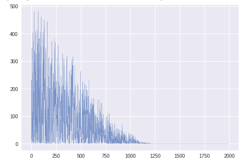
誤差
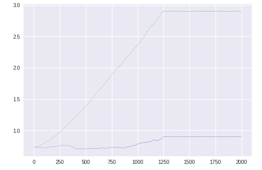
1200エポック程度で収束している。パラメータθ1,θ2
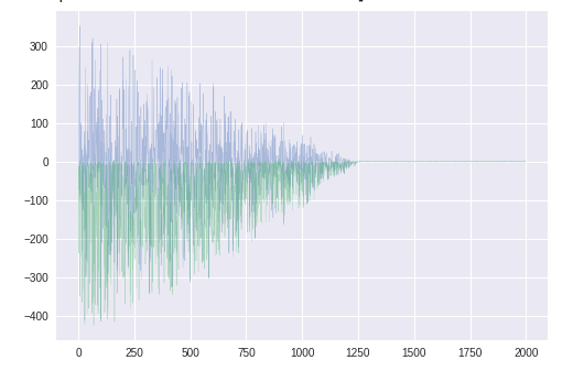
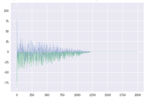
青いほうが$\theta_1$。青線が少しふらついているが、問題なく最適解に向かっているようである。勾配gt
青いほうが$\theta_1$に関する勾配。$\theta_2$とは異なり、正負に振れがある。
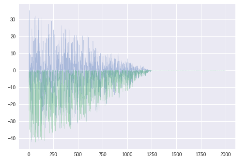
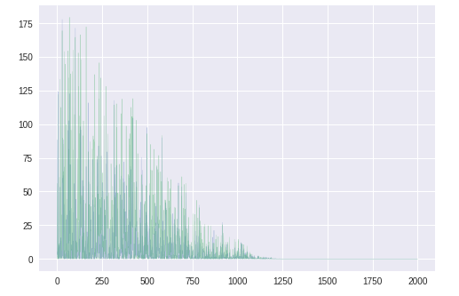
$\theta$のグラフに見えるふらつきはこのためか。勾配の平均mt
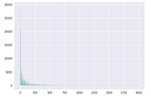
スケールが小さくなったが、形は$g_t$と類似。バイアス補正した勾配の平均mt^
学習初期のみ値が大きく、以降は元より小さくなっている。前回、0で初期化された学習初期だけ補正が強く働いている
と書いたが、やはりそのようである。
($\hat{m_t} \leftarrow \frac{m_t}{(1-\beta_1^t)}$で、$\beta_1^t$がどんどん小さくなるから、あとの方では補正が弱くなる)勾配の分散vt
同じ方向を向いているのでわかりにくいが、
$\theta_2$に対応する緑色のほうが大きい。バイアス補正した勾配の分散vt^
かなり補正されている。$\hat{m_t}$同様、後半に行くほど補正が弱まる。
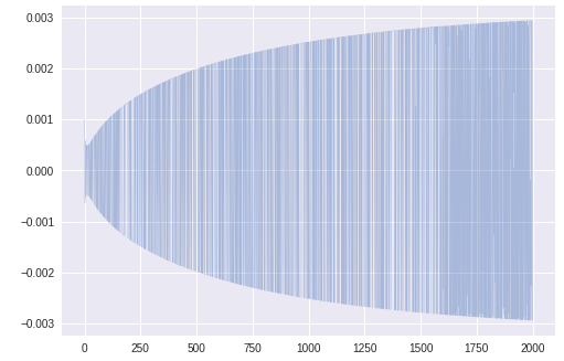
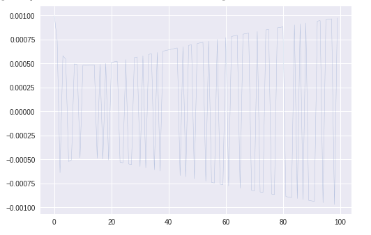
$\hat{v_t} \leftarrow \frac{v_t}{(1-\beta_2^t)}$更新幅の係数
$\theta_1$更新のステップサイズを可視化したところ、このグラフが得られた。
これは次のコードで右辺の第2項の部分である。theta_t1=theta_t_old1 -ALPHA * m_t_hat1 / (math.sqrt(v_t_hat1 + EPS))グラフを拡大すると
かなりふらついている。まとめ
- 2次元のパラメータベクトル$\vec{\theta} = (\theta_1, \theta_2) $に対して最適化を行うAdamをpythonで実装した
- 目的関数はモデル$y=\theta_1 x_1 + \theta_2 x_2$に2乗誤差を適用したもの
- パラメータ$\theta_1,\theta_2$の最適解への収束、Adamのバイアス補正の挙動等を確認できた。パラメータが複数でも問題なく動作することがわかった。
展望
- Adam以外のソルバーとの比較
- ニューラルネットワーク