- 投稿日:2019-07-07T23:25:36+09:00
[Python] 型の把握は大事です
はじめに
最近Pyhonを勉強し始めた新人です。
今回はAtCoderを解いているときにはまってしまったことについて書きたいと思います。
はまってしまった問題
以下に問題を載せます。
B - Ordinary Number問題
{1, 2, ..., n}の順列p={p1, p2, ..., pn}があります。
以下の条件を満たすようなpi(1 < i < n)がいくつあるかを出力せよ。
- pi-1, pi, pi+1 の3つの数の中で、piが2番目に小さい。
制約
- 入力はすべて整数である。
- 3 <= n <=20
- pは{1, 2, ..., n}の順列である。
考え方
pi-1, pi, pi+1の3つの数の中で、piが2番目に小さい。
すなわち以下の条件を満たせばよいと考えました。
- pi-1 < pi < pi+1 または pi-1 > pi > pi+1
また、nの最大値が20のため、全部見ていっても問題ないですね。
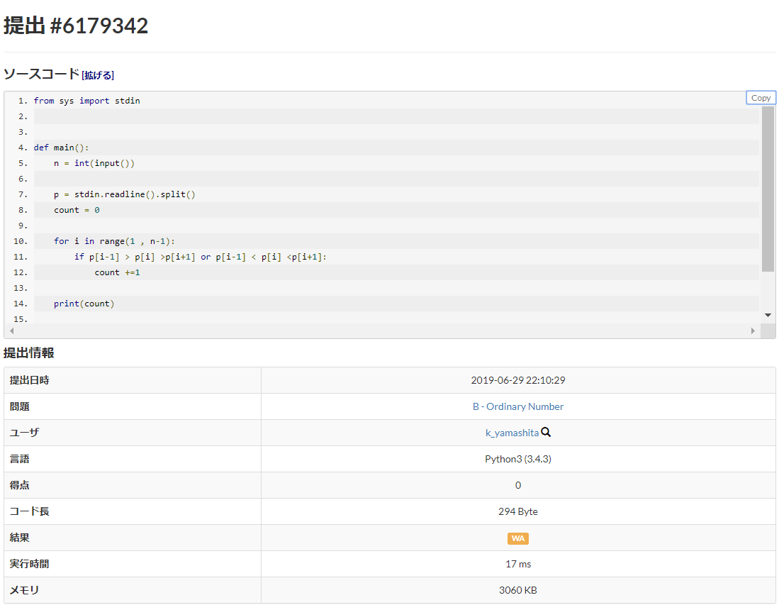
実際に書いたコード
from sys import stdin


def main():
    n = int(input())
    p = stdin.readline().split()
    count = 0
    for i in range(1 , n-1):
        if p[i-1] > p[i] >p[i+1] or p[i-1] < p[i] <p[i+1]:
            count +=1
    print(count)

if __name__ == "__main__":
    main()
入力例では、正しく出力できたので提出してみましょう。
結果
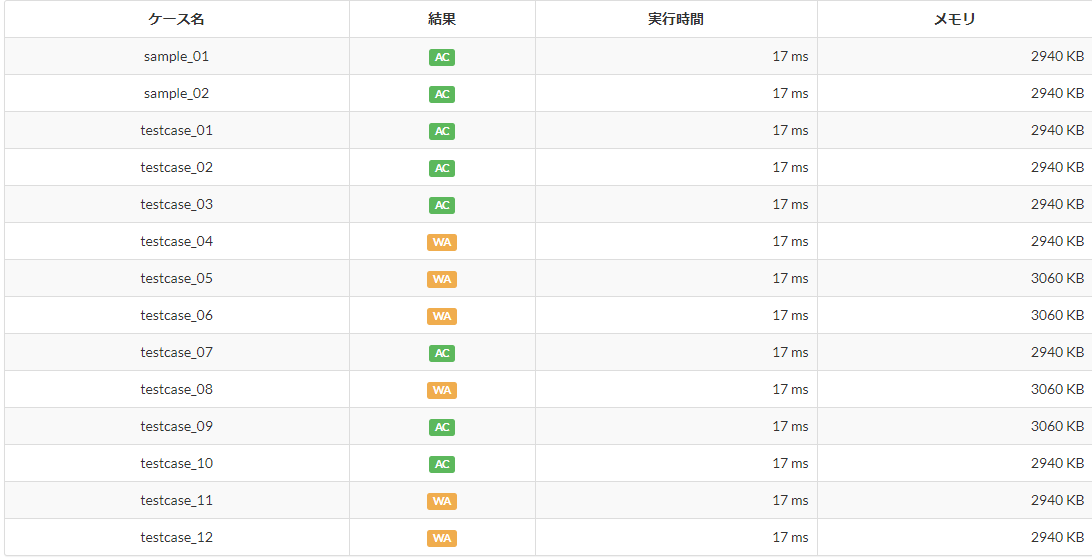
WAです。
どうやら通らないテストケースがあるようです。
コードを見直してみると、pの中身がint型ではなく、str型になっていることがわかりました。
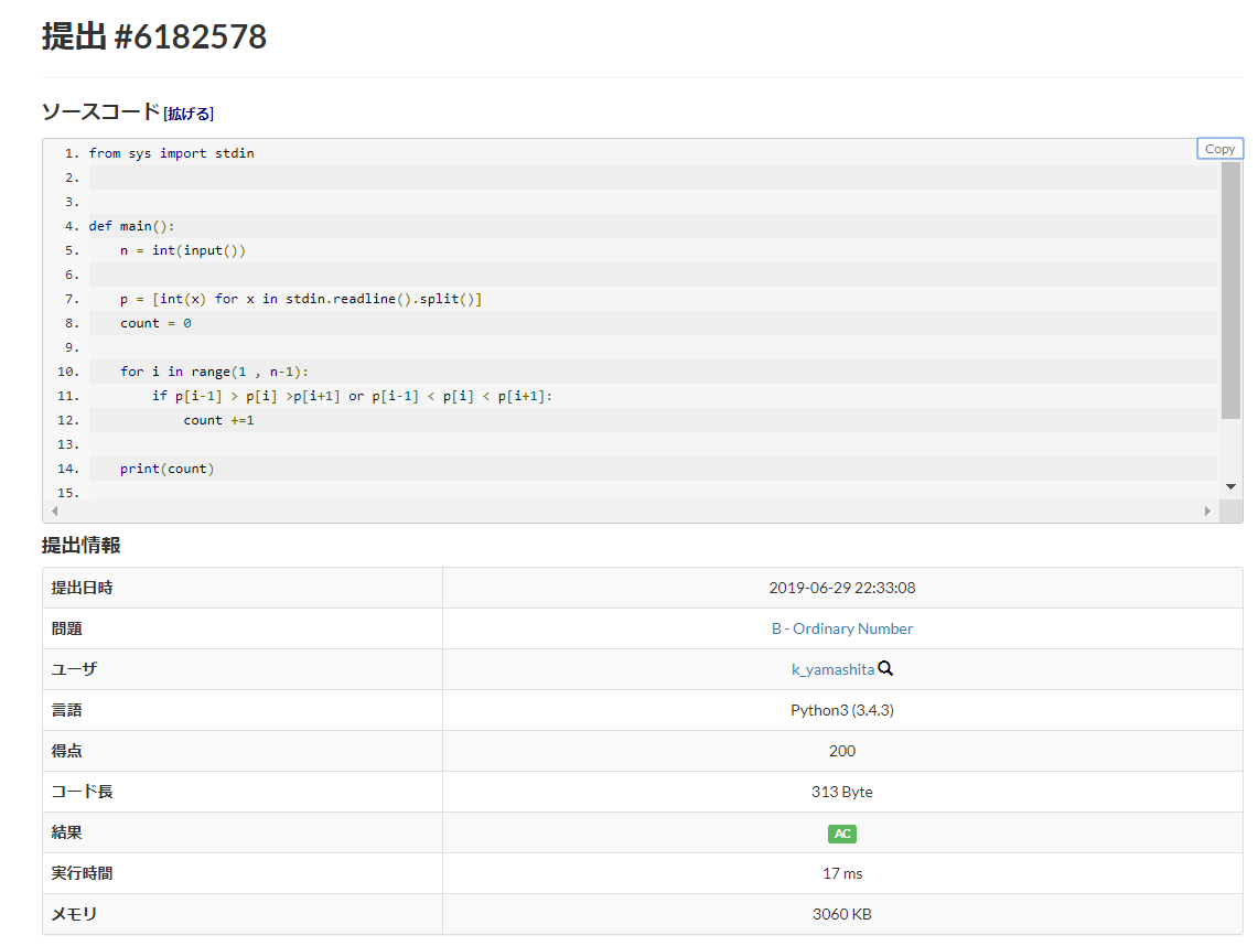
以下のように修正します。from sys import stdin def main(): n = int(input()) p = [int(x) for x in stdin.readline().split()] count = 0 for i in range(1 , n-1): if p[i-1] > p[i] >p[i+1] or p[i-1] < p[i] < p[i+1]: count +=1 print(count) if __name__ == "__main__": main()提出してみると
無事ACです!
反省
型の把握が甘かったことが今回の反省点です。
また、string型の比較である程度通ってしまったが故に、気づくのが遅くなってしまいました。ちなみに
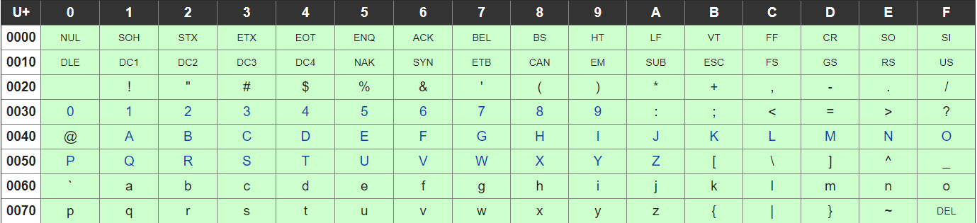
今回間違えてstring型で比較をしてしまいましたが、string型の比較はどのような挙動になるのか調べてみると、以下のサイトが見つかりました。
https://note.nkmk.me/python-str-compare/上記のサイトによると、
Python3では文字列strはUnicodeであり、文字列の大小関係(順番)は文字のUnicodeコードポイント(文字コード)で判定される。
文字列も数値などと同様に<, <=, >, >=演算子で比較できる。1文字目が同じなら2文字目、3文字目...と順番に比較される。
以下はUnicode表の一部です。
そのため、同じ桁同士だとint型と同じ結果になりますが、桁が違うと、異なる結果になってしまいますね。
- 投稿日:2019-07-07T22:53:15+09:00
SIGNATE「銀行の顧客ターゲティング」を決定木で予測してみた
はじめに
SIGNATE様が提供しているプラクティスコンペに参加してみました。
使用データは、ある銀行の顧客属性データおよび、過去のキャンペーンでの接触情報、などで、これらのデータを元に、当該のキャンペーンの結果、口座を開設したかどうかを予測します。
ねらい
今回はデータの前処理や、パラメータ設定の理解に重きを置くため、決定木のみ(ランダムフォレスト等のアンサンブル学習を使わない)でモデル作成に取り組みました。
決定木で出せる予測値の限界?とされている0.91以上を目指してみます。環境
Anaconda JupyterLab
データ分析
準備
ライブラリーのインポート
import numpy as np
import pandas as pd
from sklearn.tree import DecisionTreeClassifier as DT
from sklearn.tree import DecisionTreeClassifier, export_graphviz
from sklearn.externals.six import StringIO
from sklearn.metrics import roc_auc_score
import pydotplus
from IPython.display import Image
データの読み込み
# Path
input_path = "../input_data/"

# Set Display Max Columns
pd.set_option("display.max_columns", 50)

train = pd.read_csv(input_path + "bank/train.csv", sep=",", header=0, quotechar="\"")
test = pd.read_csv(input_path + "bank/test.csv", sep=",", header=0, quotechar="\"")
前処理
対数変換
## ヒストグラムでプロットしたときに、分布に偏りがある項目
train["log_balance"] = np.log(train.balance - train.balance.min() + 1)
train["log_duration"] = np.log(train.duration + 1)
train["log_campaign"] = np.log(train.campaign + 1)
train["log_pdays"] = np.log(train.pdays - train.pdays.min() + 1)

test["log_balance"] = np.log(test.balance - test.balance.min() + 1)
test["log_duration"] = np.log(test.duration + 1)
test["log_campaign"] = np.log(test.campaign + 1)
test["log_pdays"] = np.log(test.pdays - test.pdays.min() + 1)

drop_columns = ["id", "balance", "duration", "campaign", "pdays"]

train = train.drop(drop_columns, axis = 1)
test  = test.drop(drop_columns, axis = 1)
trainとtestに分けてしまったため、冗長な書き方に...
(trainデータに)monthを数値、datetimeを作成
# month を文字列から数値に変換
month_dict = {"jan": 1, "feb": 2, "mar": 3, "apr": 4, "may": 5, "jun": 6,
              "jul": 7, "aug": 8, "sep": 9, "oct": 10, "nov": 11, "dec": 12}
train["month_int"] = train["month"].map(month_dict)


# month と day を datetime に変換
data_datetime = train \
    .assign(ymd_str=lambda x: "2014" + "-" + x["month_int"].astype(str) + "-" + x["day"].astype(str)) \
    .assign(datetime=lambda x: pd.to_datetime(x["ymd_str"])) \
    ["datetime"].values

# datetime を int に変換する
index = pd.DatetimeIndex(data_datetime)
train["datetime_int"] = np.log(index.astype(np.int64))

# 不要な列を削除
train = train.drop(["month", "day", "month_int"], axis=1)
del data_datetime
del index
(testデータに)monthを数値、datetimeを作成
# month を文字列から数値に変換
month_dict = {"jan": 1, "feb": 2, "mar": 3, "apr": 4, "may": 5, "jun": 6,
              "jul": 7, "aug": 8, "sep": 9, "oct": 10, "nov": 11, "dec": 12}
test["month_int"] = test["month"].map(month_dict)


# month と day を datetime に変換
data_datetime = test \
    .assign(ymd_str=lambda x: "2014" + "-" + x["month_int"].astype(str) + "-" + x["day"].astype(str)) \
    .assign(datetime=lambda x: pd.to_datetime(x["ymd_str"])) \
    ["datetime"].values

# datetime を int に変換する
index = pd.DatetimeIndex(data_datetime)
test["datetime_int"] = np.log(index.astype(np.int64))

# 不要な列を削除
test = test.drop(["month", "day", "month_int"], axis=1)
del data_datetime
del index
One Hot Encoding
cat_cols = ["job", "marital", "education", "default", "housing", "loan", "contact", "poutcome"]
train_dummy = pd.get_dummies(train[cat_cols])
test_dummy = pd.get_dummies(test[cat_cols])
データ結合
train_tmp = train[["age", "datetime_int", "log_balance", "log_duration", "log_campaign", "log_pdays", "y"]]
test_tmp = test[["age", "datetime_int", "log_balance", "log_duration", "log_campaign", "log_pdays"]]


train = pd.concat([train_tmp, train_dummy], axis=1)
test = pd.concat([test_tmp, test_dummy], axis=1)
目的変数を分離
train_x = train.drop(columns=["y"])
train_y = train[["y"]]
train_x.head()
モデル作成からテストデータへの適用まで
交差検証とグリットサーチによるパラメータの最適化
from sklearn.model_selection import KFold
from sklearn import metrics
from sklearn.metrics import accuracy_score
from sklearn.model_selection import GridSearchCV
from sklearn import tree


K = 3 #今回は3分割
kf = KFold(n_splits=K, shuffle=True, random_state=17)

clf = tree.DecisionTreeClassifier(random_state=17)

# use a full grid over all parameters
param_grid = {"max_depth": [6, 7, 8, 9],
#              "max_features": ['log2', 'sqrt','auto'],
              "min_samples_split": [2, 3, 4],
              "min_samples_leaf": [15, 17, 18, 19, 20, 25, 26],
              "criterion": ["gini"]} #gini係数で評価

#次に、GridSearchCVを読んで、グリッドサーチを実行する。
tree_grid = GridSearchCV(estimator=clf,
                 param_grid = param_grid,
                 scoring="accuracy",  #metrics
                 cv = K,              #cross-validation
                 n_jobs =-1)          #number of core

tree_grid.fit(train_x,train_y) #fit

tree_grid_best = tree_grid.best_estimator_ #best estimator
print("Best Model Parameter: ",tree_grid.best_params_)
print("Best Model Score    : ",tree_grid.best_score_)
Best Model Parameter: {'criterion': 'gini', 'max_depth': 7, 'min_samples_leaf': 18, 'min_samples_split': 2}
Best Model Score : 0.9002875258035977*tree_gridではなく、tree_grid_bestを使用すること。交差検証の評価から得た最適解が、tree_grid_bestの方に入っているので(モデル性能が悪くなり、ここで、かなり足止めを食らった...)
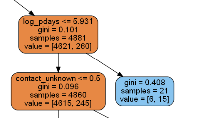
col_name = list(train_x.columns.values)

dot_data = StringIO()
export_graphviz(tree_grid_best, out_file=dot_data, feature_names=col_name, filled=True, rounded=True)
tree_graph = pydotplus.graph_from_dot_data(dot_data.getvalue())

tree_graph.progs = {"dot": u"graphvizのdot.exeがあるパスを指定"} #windowsでは必要

tree_graph.write_png('tree.png') #画像の保存
Image(tree_graph.create_png())
読み方としては、青色の濃い部分は目的変数である、定額預金の申し込みが有(yes) が多い分類、逆にオレンジ色は少ないということになります。
上図の青色のboxを例にあげると、log_pdays<=5.931 ではない(つまり log_pdays> 5.931)の区分に青色が多い。また、gini係数の値が0に近いほど、よく分離できている(条件式として優秀)ということが分かる。
改めてAUCでモデルの評価(あまり意味がないが...)
pred = tree_grid_best.predict_proba(train_x)[:, 1]
roc_auc_score(train_y, pred)
0.9124593798479221
テストデータに適用
pred_test = tree_grid_best.predict_proba(test)[:, 1] #ちゃんとtree_grid_bestに投稿用にデータを整形
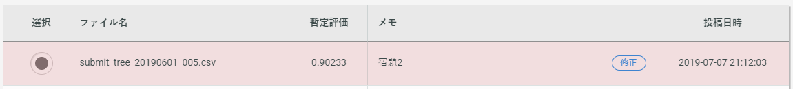
test_for_id = pd.read_csv(input_path + "bank/test.csv", sep=",", header=0, quotechar="\"")
ID = np.array(test_for_id[["id"]]).astype(int)

my_solution = pd.DataFrame(pred_test, ID).reset_index()

# Submit File
my_solution.to_csv(
    path_or_buf="../submit/submit_tree_20190601_005.csv", # 出力先
    sep=",",                                            # 区切り文字
    index=False,                                        # indexの出力有無
    header=False                                        # headerの出力有無
)
結果
0.91までまだまだ。さらなる調整が必要...
参考・引用
以下を参考にさせて頂きました。
・https://futurismo.biz/archives/6801/
・https://github.com/mamurata0924/signate_bank_customer_targeting
・https://qiita.com/shinya7y/items/d38716ee4c81b3806eea


- 投稿日:2019-07-07T22:53:15+09:00
SIGNATE「銀行の顧客ターゲティング」を決定木だけで予測してみた
はじめに
SIGNATE様が提供しているプラクティスコンペに参加してみました。
使用データは、ある銀行の顧客属性データおよび、過去のキャンペーンでの接触情報、などで、これらのデータを元に、当該のキャンペーンの結果、口座を開設したかどうかを予測します。
ねらい
今回はデータの前処理や、パラメータ設定の理解に重きを置くため、決定木のみ(ランダムフォレスト等のアンサンブル学習を使わない)でモデル作成に取り組みました。
決定木で出せる予測値の限界?とされている0.91以上を目指してみます。環境
Anaconda JupyterLab
データ分析
準備
ライブラリーのインポート
import numpy as np
import pandas as pd
from sklearn.tree import DecisionTreeClassifier as DT
from sklearn.tree import DecisionTreeClassifier, export_graphviz
from sklearn.externals.six import StringIO
from sklearn.metrics import roc_auc_score
import pydotplus
from IPython.display import Image
データの読み込み
# Path
input_path = "../input_data/"

# Set Display Max Columns
pd.set_option("display.max_columns", 50)

train = pd.read_csv(input_path + "bank/train.csv", sep=",", header=0, quotechar="\"")
test = pd.read_csv(input_path + "bank/test.csv", sep=",", header=0, quotechar="\"")
前処理
対数変換
## ヒストグラムでプロットしたときに、分布に偏りがある項目
train["log_balance"] = np.log(train.balance - train.balance.min() + 1)
train["log_duration"] = np.log(train.duration + 1)
train["log_campaign"] = np.log(train.campaign + 1)
train["log_pdays"] = np.log(train.pdays - train.pdays.min() + 1)

test["log_balance"] = np.log(test.balance - test.balance.min() + 1)
test["log_duration"] = np.log(test.duration + 1)
test["log_campaign"] = np.log(test.campaign + 1)
test["log_pdays"] = np.log(test.pdays - test.pdays.min() + 1)

drop_columns = ["id", "balance", "duration", "campaign", "pdays"]

train = train.drop(drop_columns, axis = 1)
test  = test.drop(drop_columns, axis = 1)
trainとtestに分けてしまったため、冗長な書き方に...
(trainデータに)monthを数値、datetimeを作成
# month を文字列から数値に変換
month_dict = {"jan": 1, "feb": 2, "mar": 3, "apr": 4, "may": 5, "jun": 6,
              "jul": 7, "aug": 8, "sep": 9, "oct": 10, "nov": 11, "dec": 12}
train["month_int"] = train["month"].map(month_dict)


# month と day を datetime に変換
data_datetime = train \
    .assign(ymd_str=lambda x: "2014" + "-" + x["month_int"].astype(str) + "-" + x["day"].astype(str)) \
    .assign(datetime=lambda x: pd.to_datetime(x["ymd_str"])) \
    ["datetime"].values

# datetime を int に変換する
index = pd.DatetimeIndex(data_datetime)
train["datetime_int"] = np.log(index.astype(np.int64))

# 不要な列を削除
train = train.drop(["month", "day", "month_int"], axis=1)
del data_datetime
del index
(testデータに)monthを数値、datetimeを作成
# month を文字列から数値に変換
month_dict = {"jan": 1, "feb": 2, "mar": 3, "apr": 4, "may": 5, "jun": 6,
              "jul": 7, "aug": 8, "sep": 9, "oct": 10, "nov": 11, "dec": 12}
test["month_int"] = test["month"].map(month_dict)


# month と day を datetime に変換
data_datetime = test \
    .assign(ymd_str=lambda x: "2014" + "-" + x["month_int"].astype(str) + "-" + x["day"].astype(str)) \
    .assign(datetime=lambda x: pd.to_datetime(x["ymd_str"])) \
    ["datetime"].values

# datetime を int に変換する
index = pd.DatetimeIndex(data_datetime)
test["datetime_int"] = np.log(index.astype(np.int64))

# 不要な列を削除
test = test.drop(["month", "day", "month_int"], axis=1)
del data_datetime
del index
One Hot Encoding
cat_cols = ["job", "marital", "education", "default", "housing", "loan", "contact", "poutcome"]
train_dummy = pd.get_dummies(train[cat_cols])
test_dummy = pd.get_dummies(test[cat_cols])
データ結合
train_tmp = train[["age", "datetime_int", "log_balance", "log_duration", "log_campaign", "log_pdays", "y"]]
test_tmp = test[["age", "datetime_int", "log_balance", "log_duration", "log_campaign", "log_pdays"]]


train = pd.concat([train_tmp, train_dummy], axis=1)
test = pd.concat([test_tmp, test_dummy], axis=1)
目的変数を分離
train_x = train.drop(columns=["y"]) train_y = train[["y"]]train_x.head()
モデル作成からテストデータへの適用まで
交差検証とグリットサーチによるパラメータの最適化
from sklearn.model_selection import KFold
from sklearn import metrics
from sklearn.metrics import accuracy_score
from sklearn.model_selection import GridSearchCV
from sklearn import tree


K = 3 #今回は3分割
kf = KFold(n_splits=K, shuffle=True, random_state=17)

clf = tree.DecisionTreeClassifier(random_state=17)

# use a full grid over all parameters
param_grid = {"max_depth": [6, 7, 8, 9],
#              "max_features": ['log2', 'sqrt','auto'],
              "min_samples_split": [2, 3, 4],
              "min_samples_leaf": [15, 17, 18, 19, 20, 25, 26],
              "criterion": ["gini"]} #gini係数で評価

#次に、GridSearchCVを読んで、グリッドサーチを実行する。
tree_grid = GridSearchCV(estimator=clf,
                 param_grid = param_grid,
                 scoring="accuracy",  #metrics
                 cv = K,              #cross-validation
                 n_jobs =-1)          #number of core

tree_grid.fit(train_x,train_y) #fit

tree_grid_best = tree_grid.best_estimator_ #best estimator
print("Best Model Parameter: ",tree_grid.best_params_)
print("Best Model Score    : ",tree_grid.best_score_)
Best Model Parameter: {'criterion': 'gini', 'max_depth': 7, 'min_samples_leaf': 18, 'min_samples_split': 2}
Best Model Score : 0.9002875258035977*tree_gridではなく、tree_grid_bestを使用すること。交差検証の評価から得た最適解が、tree_grid_bestの方に入っているので(モデル性能が悪くなり、ここで、かなり足止めを食らった...)
col_name = list(train_x.columns.values)

dot_data = StringIO()
export_graphviz(tree_grid_best, out_file=dot_data, feature_names=col_name, filled=True, rounded=True)
tree_graph = pydotplus.graph_from_dot_data(dot_data.getvalue())

tree_graph.progs = {"dot": u"graphvizのdot.exeがあるパスを指定"} #windowsでは必要

tree_graph.write_png('tree.png') #画像の保存
Image(tree_graph.create_png())
読み方としては、青色の濃い部分は目的変数である、定額預金の申し込みが有(yes) が多い分類、逆にオレンジ色は少ないということになります。
上図の青色のboxを例にあげると、log_pdays<=5.931 ではない(つまり log_pdays> 5.931)の区分に青色が多い。また、gini係数の値が0に近いほど、よく分離できている(条件式として優秀)ということが分かる。
改めてAUCでモデルの評価(あまり意味がないが...)
pred = tree_grid_best.predict_proba(train_x)[:, 1]
roc_auc_score(train_y, pred)
0.9124593798479221
テストデータに適用
pred_test = tree_grid_best.predict_proba(test)[:, 1] #ちゃんとtree_grid_bestに投稿用にデータを整形
test_for_id = pd.read_csv(input_path + "bank/test.csv", sep=",", header=0, quotechar="\"")
ID = np.array(test_for_id[["id"]]).astype(int)

my_solution = pd.DataFrame(pred_test, ID).reset_index()

# Submit File
my_solution.to_csv(
    path_or_buf="../submit/submit_tree_20190601_005.csv", # 出力先
    sep=",",                                            # 区切り文字
    index=False,                                        # indexの出力有無
    header=False                                        # headerの出力有無
)
結果
0.91までまだまだ。さらなる調整が必要...
参考・引用
以下を参考にさせて頂きました。
・https://futurismo.biz/archives/6801/
・https://github.com/mamurata0924/signate_bank_customer_targeting
・https://qiita.com/shinya7y/items/d38716ee4c81b3806eea
- 投稿日:2019-07-07T22:41:23+09:00
Django + Heroku + AWS S3で画像表示させる方法
概要
Djangoアプリで画像をS3に保存し、アプリに表示させる方法を書いてみます。
想定している処理は、①ユーザーが画像投稿→②S3に保存→③S3からアプリに画像表示です。なお、環境は
Python 3.7.3、Django 2.2になります。1. AWS設定
1-1. AWS登録
S3を使用するのに、AWSアカウントが必要になりますので、お持ちでない方はAWS Signupからご登録ください。
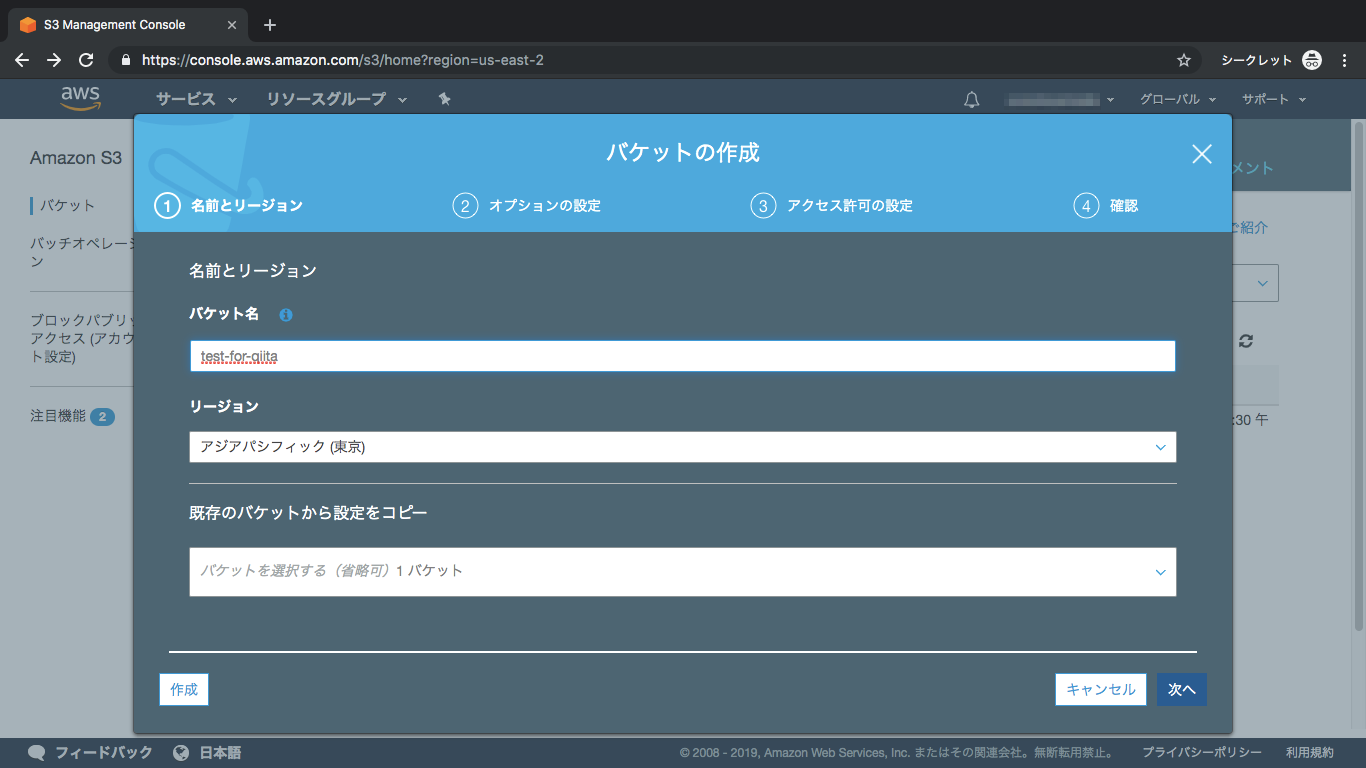
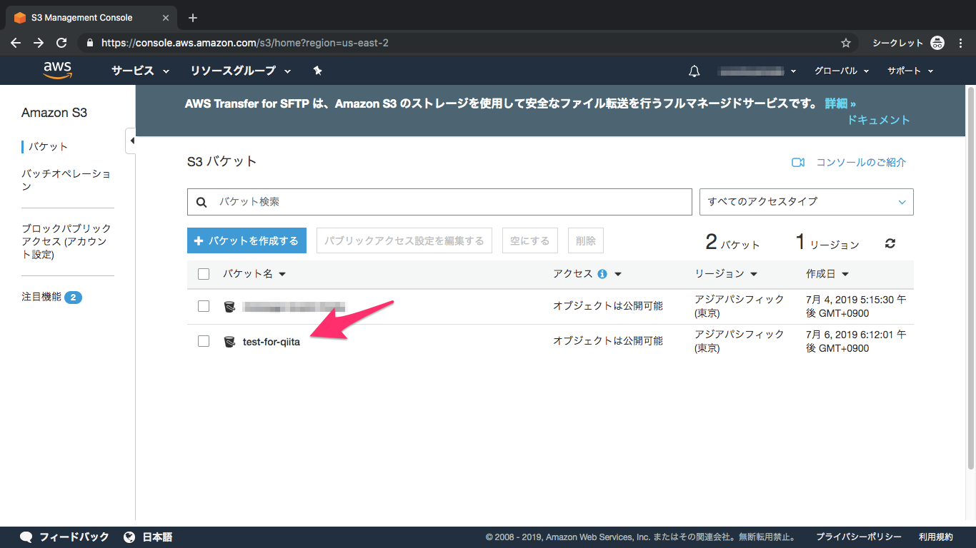
1-2. バケット作成
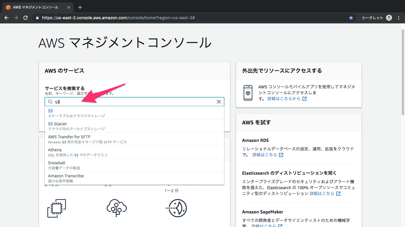
①S3を検索してクリック
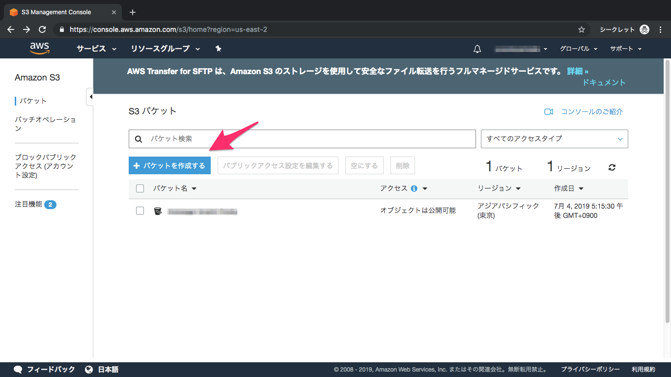
②バケット作成
③バケット名とリージョンを選択
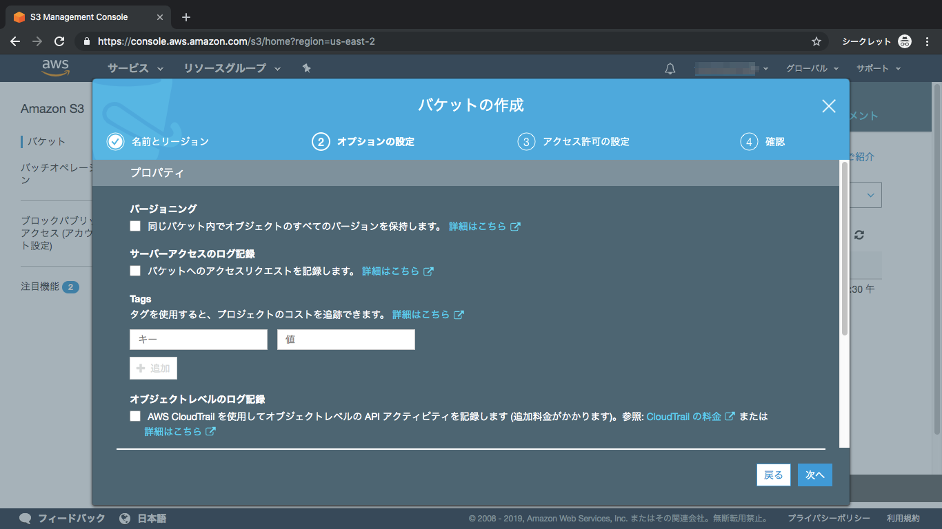
④オプションなし
オプションですが、今回は設定しません
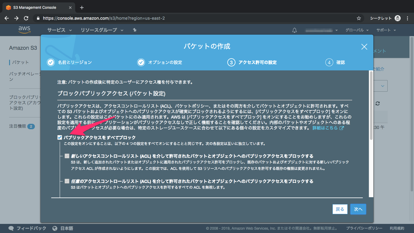
⑤アクセス権限
こちらの項目を外してください、初期設定ではブロックされてしまいます
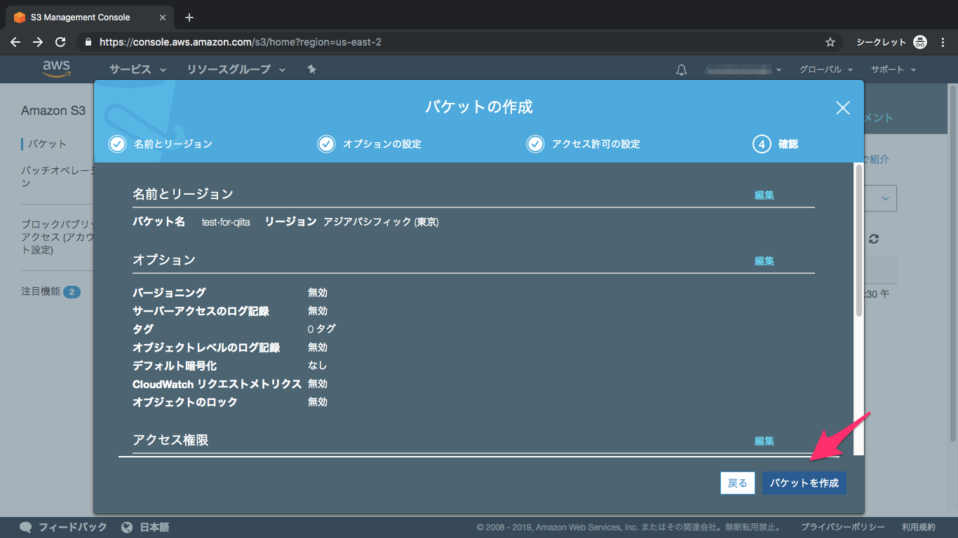
⑥内容を確認して作成
⑦バケット完成
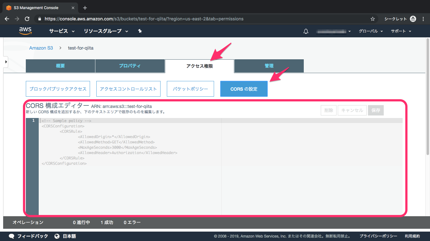
1-3. CORS設定
①CORSの設定に移動
作成したバケットをクリックし、「アクセス制限」の「CORSの設定」に移動します
②CORS構成エディターに追加
下記のように追加してください
CORS<?xml version="1.0" encoding="UTF-8"?> <CORSConfiguration xmlns="http://s3.amazonaws.com/doc/2006-03-01/"> <CORSRule> <AllowedOrigin>*</AllowedOrigin> <AllowedMethod>GET</AllowedMethod> <AllowedMethod>POST</AllowedMethod> <AllowedMethod>PUT</AllowedMethod> <AllowedHeader>*</AllowedHeader> </CORSRule> </CORSConfiguration>参照:
Cross-Origin Resource Sharing (CORS)
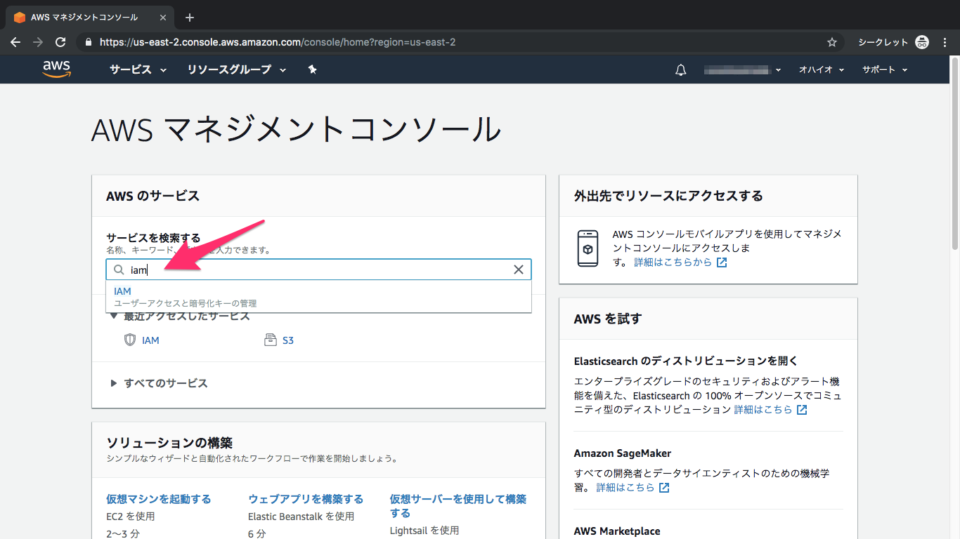
Direct to S3 File Uploads in Python | S3 Setup1-4. IAM設定
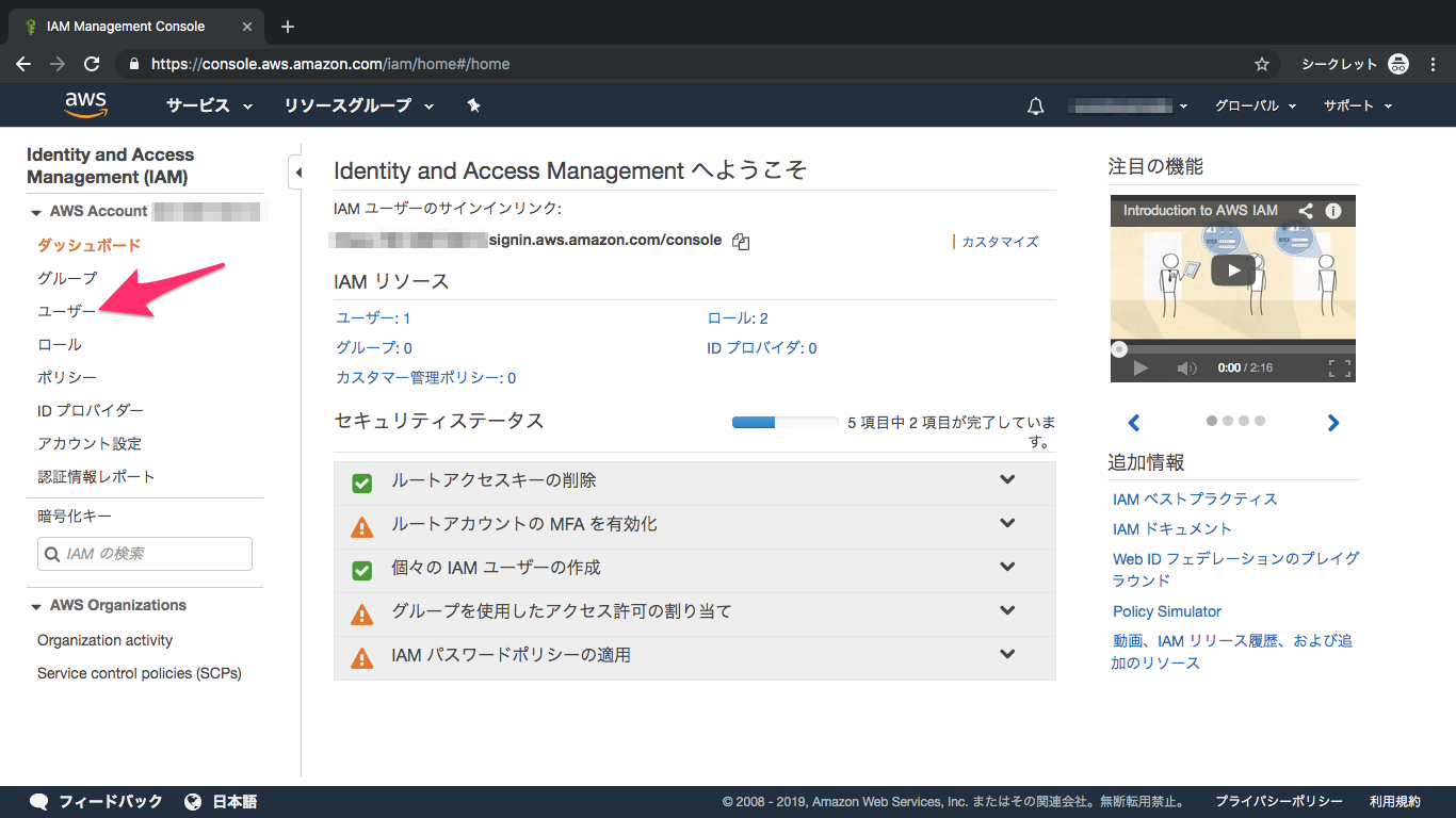
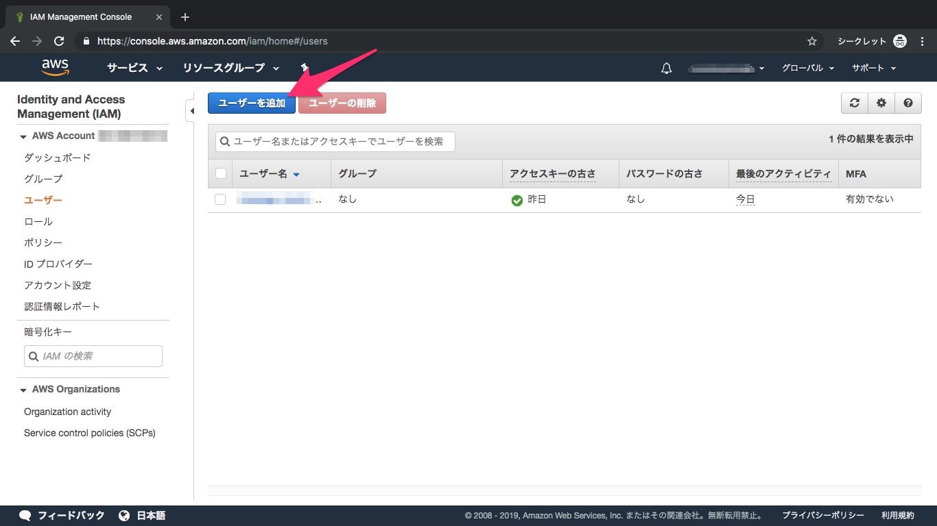
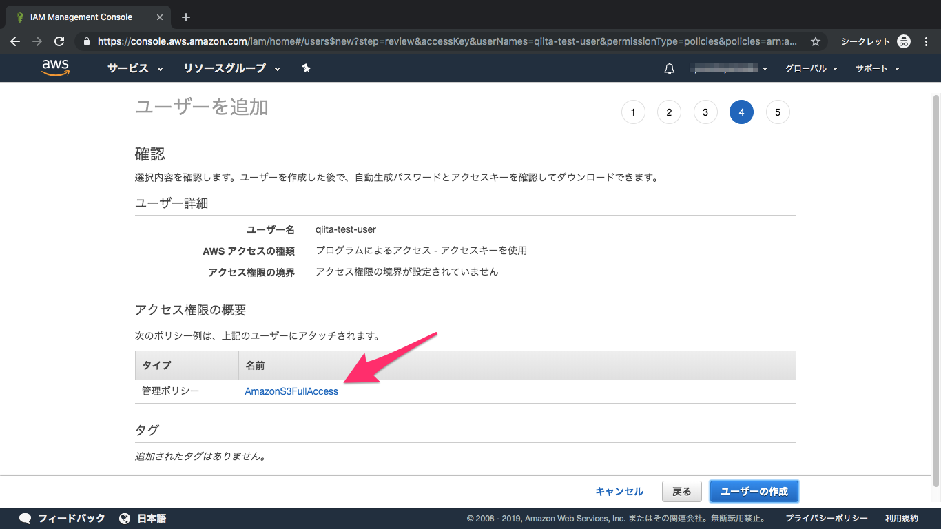
①IAMを検索してクリック
②ユーザーをクリック
③ユーザー追加をクリック
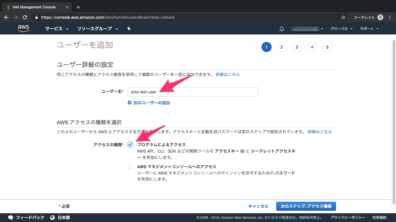
④ユーザー名を入力、プログラムによるアクセスをチェック
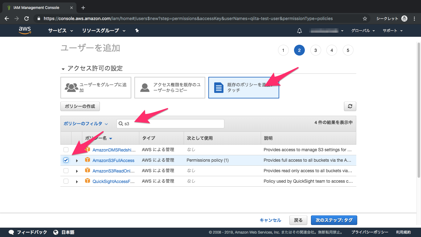
⑤アクセス許可
S3を検索し、AmazonS3FullAccessにチェック
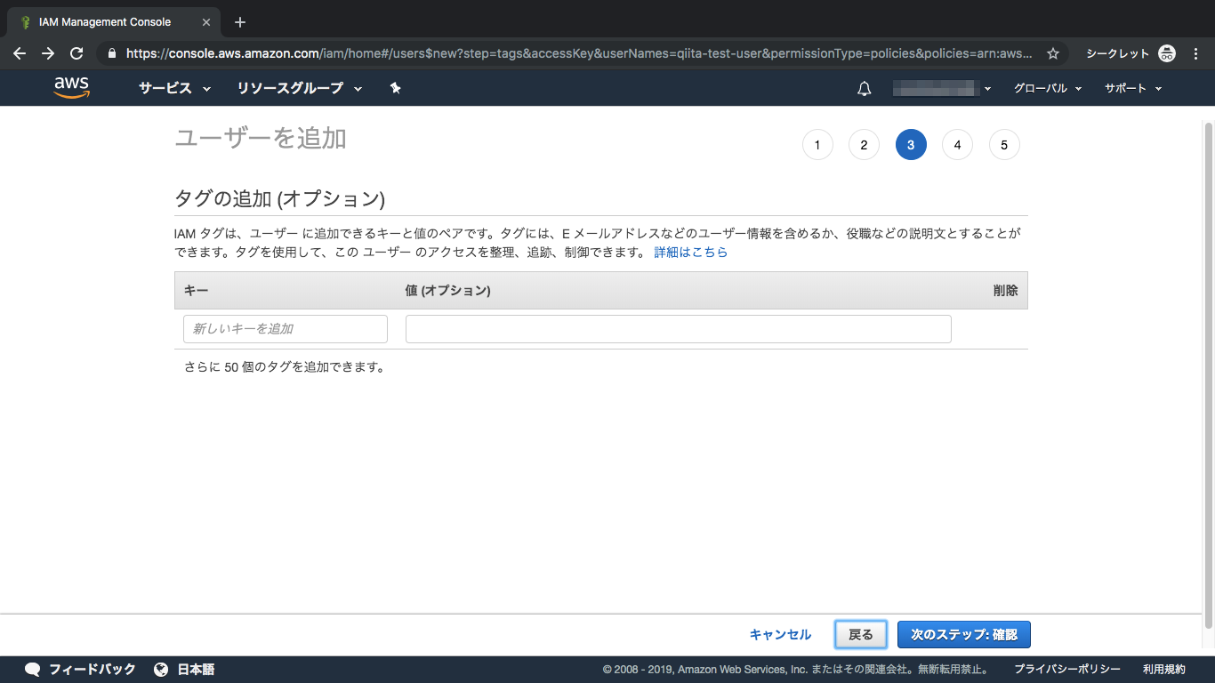
⑥オプションなし
オプションですが、今回は設定しません
⑦内容を確認して作成
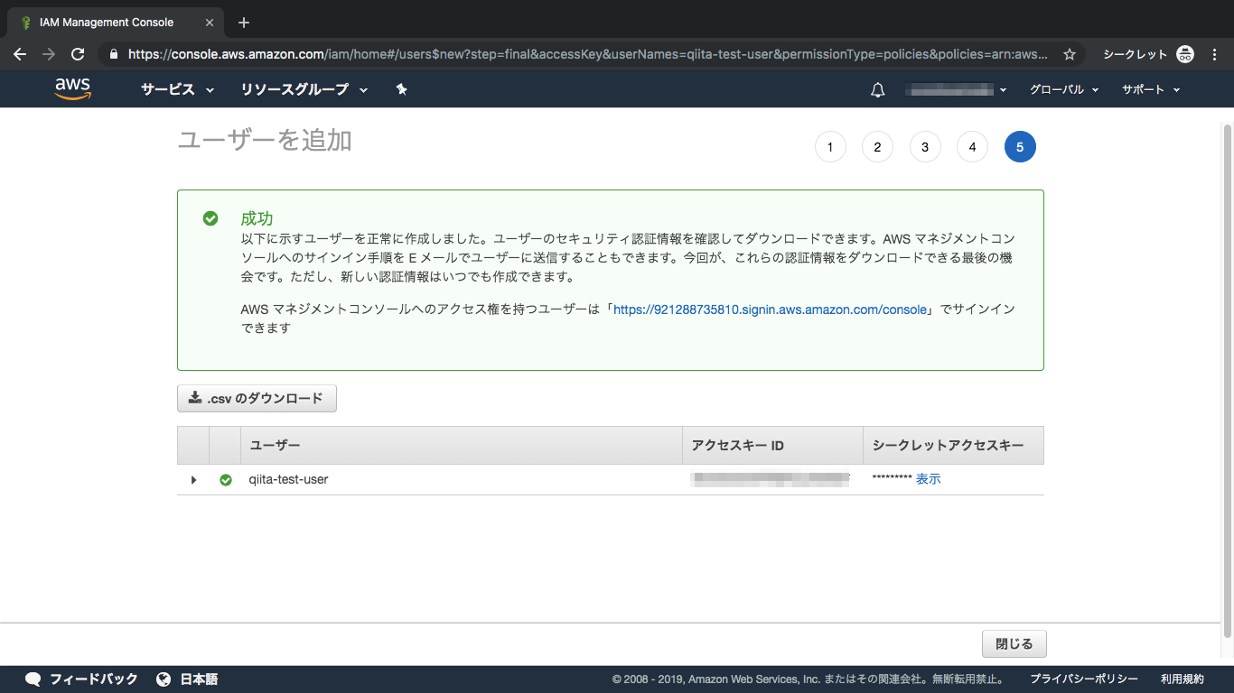
⑧IAM設定完了
後ほど、
アクセスキーIDとシークレットアクセスキーを使いますので、画面を閉じないでください
参照:IAMとは
2. アプリ設定
2-1. インストール
①django-storagesインストール
terminal$ pip install django-storages参照:django-storages | Amazon S3
②boto3インストール
terminal$ pip install boto3参照:
Boto 3 Documentation
AWS SDK for Python (Boto3)2-2. settings.py設定
下記のように追加してください
settings.pyINSTALLED_APPS = [ 'django.contrib.admin', 'django.contrib.auth', 'django.contrib.contenttypes', 'django.contrib.sessions', 'django.contrib.messages', 'django.contrib.staticfiles', 'your_app_name', 'storages', #追加 ] #追加 AWS_ACCESS_KEY_ID = os.environ['AWS_ACCESS_KEY_ID'] AWS_SECRET_ACCESS_KEY = os.environ['AWS_SECRET_ACCESS_KEY'] AWS_STORAGE_BUCKET_NAME = os.environ['AWS_STORAGE_BUCKET_NAME'] DEFAULT_FILE_STORAGE = 'storages.backends.s3boto.S3BotoStorage' S3_URL = 'http://%s.s3.amazonaws.com/' % AWS_STORAGE_BUCKET_NAME MEDIA_URL = S3_URL AWS_S3_FILE_OVERWRITE = False AWS_DEFAULT_ACL = None2-3. 環境変数
Herokuの環境変数を3つ設定します。
①AWS_ACCESS_KEY_IDと②AWS_SECRET_ACCESS_KEYは、IAMユーザーを追加した際に表示された、アクセスキーIDとシークレットアクセスキーになります。
③AWS_STORAGE_BUCKET_NAMEは作成したバケット名です。terminal$ heroku config:set AWS_ACCESS_KEY_ID="ご自身のアクセスキーIDを記入" $ heroku config:set AWS_SECRET_ACCESS_KEY="ご自身のシークレットアクセスキーを記入" $ heroku config:set AWS_STORAGE_BUCKET_NAME="ご自身のバケット名を記入"参照:
Configuration and Config Vars | Heroku
Django Docs | Deployment checklist2-4. requirements.txt
インストールしたモジュールを
requirements.txtに追加します。terminal$ pip freeze > requirements.txt2-5. local_settings.py設定
もし
local_settings.pyを使用している場合は、下記を参考にしてください。ローカル環境では
MEDIA_ROOTで指定したディレクトリから読み込み、HerokuではS3から読み込むことができます。settings.py### 省略 ### DEBUG = False ALLOWED_HOSTS = ['*'] INSTALLED_APPS = [ 'django.contrib.admin', 'django.contrib.auth', 'django.contrib.contenttypes', 'django.contrib.sessions', 'django.contrib.messages', 'django.contrib.staticfiles', 'your_app_name', 'storages', ] ### 省略 ### MEDIA_ROOT = os.path.join(BASE_DIR, 'media') MEDIA_URL = '/media/' try: from .local_settings import * except ImportError: pass if not DEBUG: SECRET_KEY = os.environ['SECRET_KEY'] AWS_ACCESS_KEY_ID = os.environ['AWS_ACCESS_KEY_ID'] AWS_SECRET_ACCESS_KEY = os.environ['AWS_SECRET_ACCESS_KEY'] AWS_STORAGE_BUCKET_NAME = os.environ['AWS_STORAGE_BUCKET_NAME'] DEFAULT_FILE_STORAGE = 'storages.backends.s3boto.S3BotoStorage' S3_URL = 'http://%s.s3.amazonaws.com/' % AWS_STORAGE_BUCKET_NAME MEDIA_URL = S3_URL AWS_S3_FILE_OVERWRITE = False AWS_DEFAULT_ACL = None import django_heroku django_heroku.settings(locals()) db_from_env = dj_database_url.config(conn_max_age=600, ssl_require=True) DATABASES['default'].update(db_from_env)local_settings.pyimport os SECRET_KEY = 'ご自身のSECRET_KEYを記入' BASE_DIR = os.path.dirname(os.path.dirname(os.path.abspath(__file__))) DATABASES = { 'default': { 'ENGINE': 'django.db.backends.sqlite3', 'NAME': os.path.join(BASE_DIR, 'db.sqlite3'), } } DEBUG = True最後に
Herokuでのデプロイが曖昧でしたら、下記の記事も参考にしてみてください。
以上
- 投稿日:2019-07-07T22:35:56+09:00
ビットシリアル SIMD シミュレータ
目的
通常、我々が目にする機械(パソコン、携帯電話、家電製品など)は多いと 64bit,
少ない場合でも 8bit のデータバス幅の CPU を使用しています。しかし、世の中には 1bit の CPU というのもあります。
かつて、「複数ビット幅の CPU で動作する計算機と複数の 1bit CPU とを比較すると後者の方がコストパフォーマンス面で有利である」という理由で超並列計算機の CPU として採用されていた時代もありました(参考)。
実装コストが低さは FPGA 上で並列計算機を構成するのにも適しているのではないかと考えました。とはいえ 1bit CPU などというものを触った経験がないので、まずはシミュレータを作って動かしてみます。ネタばらしをすると、コネクションマシン(CM-1)のビットシリアルプロセッサを真似ています。
ALU
3入力ビットー2出力ビットの ALU を用います。
入力ビット数・出力ビット数が少ないので、この ALU の演算内容はこの上なくユニバーサルな形式です。つまり、3入力ビットのあらゆる組み合わせ(といっても8通りしかない)について、2出力がどうなるかを2つの真理値表で与えます。コネクションマシンは 16 個のビットシリアルプロセッサを 1 チップに実装していましたが、ここでは 64 個のプロセッサの ALU を一つの関数で書いています。少なくとも 64 個のプロセッサを同時に SIMD で動かす想定です。
1 bit CPU といってもビット間演算が一切できない 64bit CPU ではないか、と言われてしまいそうではあります。
def alu64(a, b, f, op_s, op_c):
    u'''
    A, B, F の値と真理値表を元に S, C の値を決定する。
    Args:
        a : A レジスタ (64bit) の値
        b : B レジスタ (64bit) の値
        f : F レジスタ (64bit) の値
        op_s : S を決定する真理値表 (8bit)
        op_c : C を決定する真理値表 (8bit)
    Return:
        真理値表に従って決定した値 S, C
    '''
    # A, B, F をデコード
    selector = [0] * 8
    selector[0] = ~a & ~b & ~f
    selector[1] = ~a & ~b &  f
    selector[2] = ~a &  b & ~f
    selector[3] = ~a &  b &  f
    selector[4] =  a & ~b & ~f
    selector[5] =  a & ~b &  f
    selector[6] =  a &  b & ~f
    selector[7] =  a &  b &  f
    # 真理値表に従って S, C を決定
    s = 0
    c = 0
    for i in range(0, 8):
        if (op_s & (1 << i)) != 0:
            s |= selector[i]
        if (op_c & (1 << i)) != 0:
            c |= selector[i]
    return s, c
コネクションマシンの場合、フラグレジスタ上の値が 0 か 1 かで値を更新する・しないを切り替える機能があります。これを用いて、複数ある CPU をそれぞれ別の処理に割り当てることも可能です。
def context_switch(x, y, context, context_value):
    u'''context の各ビットを context_value と比較し、
    一致するなら x のビットを、一致しないなら y のビットを採用した値を返す。
    Args:
        x : 64bit の値
        y : 64bit の値
        context: 各ビットの条件分岐を表す 64bit 値
        context_value : context が 1 のとき x を採用するなら True
    Returns:
        context, context_value に従って採用した x または y の
        各ビットからなる 64bit 値
    '''
    return ((context & x) | (~context & y)
            if context_value else
            (~context & x) | (context & y))
CPU は3つの ALU サイクルで動作します。
- LOADA - メモリ上の値を A レジスタに読み込み、参照フラグ値を読み込む。同時に真理値表の一方を保持する。
- LOADB - メモリ上の値を B レジスタに読み込み、条件フラグ値を読み込む。同時に真理値表のもう一方を保持する。
- STORE - 保持した真理値表に従って値を生成し、A レジスタ読み込み元メモリに書き戻す。同時にフラグ値を更新する。
ということが巷にあるコネクションマシンの解説書に書いてあったので、それに従ってメソッド m_load_a, m_load_b, m_store として実装しました。
また、CPU なのでリセットも必要でしょう。フラグレジスタを 0 クリアする処理として reset メソッドを実装しました。get_flag64 / set_flag64 は外部からフラグレジスタを読み書きするためのメソッドです。
フラグレジスタの一つはルータとの入出力として使う予定です。1 bit しかない値を入出力に使うのは奇異に感じられるかもしれません。しかし、この CPU は独立して動作することはできず、外部から LOADA / LOADB / STORE のサイクルで外部のコントローラから呼び出してもらう必要があります。このコントローラはルータに対しても「CPU がデータを送りたいのでよろしく」とタイミングを指示できるので、その指示に合わせて CPU 側からデータを書き込むようにコントローラが CPU を操作すればよいわけです。受信についても同様です。
また、ビットマップディスプレイを用意してフラグの特定ビットを表示するとデバッグ(特にルータがらみのデバッグ)に便利です。大量にプロセッサを並べたものを俯瞰するのは GUI 上での表示なしでは厳しいものがあります。class Processor64: def __init__(self, memory): u'''64 CPU 分のインスタンスを作成する。 Args: memory : 外部メモリ ''' self._memory = memory # 外部メモリ self._flags = [0] * 64 # フラグレジスタ (64bit * 64) # 以下、演算動作のための内部レジスタ self._reg_addr_a = 0 self._reg_a = 0 # メモリから読み出した値 A (64bit) self._reg_b = 0 # メモリから読み出した値 B (64bit) self._reg_f = 0 # フラグから読み出した値 F (64bit) self._wire_s = 0 # ALU 計算結果 S (64bit) デバッグ用 self._wire_c = 0 # ALU 計算結果 C (64bit) デバッグ用 self._reg_context = 0 # コンテキスト判断値 (64bit) self._reg_op_s = 0 # ALU に与えられる真理値表 (8bit) self._reg_op_c = 0 # ALU に与えられる真理値表 (8bit) def dump_flags(self): u'''フラグレジスタの値を表示する。 ''' for i in range(0, len(self._flags)): if self._flags[i] == 0: continue print('flag[{:2x}]: {:064b}'.format( i, self._flags[i] & 0xffffffffffffffff)) def dump_regs(self): u'''レジスタの値を表示する。 ''' print(' A : {:064b}'.format(self._reg_a & 0xffffffffffffffff)) print(' B : {:064b}'.format(self._reg_b & 0xffffffffffffffff)) print(' F : {:064b}'.format(self._reg_f & 0xffffffffffffffff)) print(' S : {:064b}'.format(self._wire_s & 0xffffffffffffffff)) print(' C : {:064b}'.format(self._wire_c & 0xffffffffffffffff)) print(' context: {:064b}'.format( self._reg_context & 0xffffffffffffffff)) def dump_ops(self): u'''真理値表の値を表示する。 ''' print('A B F | S C') print('-----------') for a in range(0, 2): for b in range(0, 2): for f in range(0, 2): i = (a << 2) | (b << 1) | f print('{} {} {} | {} {}'.format( a, b, f, 1 if self._reg_op_s & (1 << i) else 0, 1 if self._reg_op_c & (1 << i) else 0)) def dump(self): u'''デバッグダンプ。 ''' self.dump_flags() self.dump_regs() self.dump_ops() def reset(self): u'''フラグレジスタをリセットする。 ''' self._flags = [0] * 64 def get_flag64(self, read_flag): u'''フラグレジスタ上の値を 64 プロセッサ分まとめて返す。 Args: read_flag : 読み出すフラグレジスタを指定するインデックス Returns: 読み出した値 (64bit) ''' return self._flags[read_flag] def set_flag64(self, write_flag, value64): u'''フラグレジスタ上の値を 64 プロセッサ分まとめて設定する。 Args: write_flag : 読み出すフラグレジスタを指定するインデックス value64 : 設定する値 (64bit) ''' self._flags[write_flag] = value64 def m_load_a(self, addr, read_flag, op_s): u''' LOADA : read memory operand A, read flag operand, latch one truth table Args: addr : A レジスタに読み込むメモリのアドレス read_flag : F レジスタに読み込むフラグのインデックス op_s : ALU に与える S 真理値表 (8bit) ''' self._flags[0] = 0 # 0 番目のフラグの値は常に 0 self._reg_addr_a = addr self._reg_a = self._memory[addr] self._reg_f = self._flags[read_flag] self._reg_op_s = op_s def m_load_b(self, addr, context_flag, op_c): u''' LOADB : read memory operand B, read condition flag, latch other truth table Args: addr : B レジスタに読み込むメモリのアドレス context_flag : context レジスタに読み込むフラグのインデックス op_c : ALU に与える C 真理値表 (8bit) ''' self._reg_b = self._memory[addr] self._reg_context = self._flags[context_flag] self._reg_op_c = op_c def m_store(self, write_flag, context_value): u''' STORE : store memory operand A, store result flag Args: write_flag : C 値書き込み先フラグのインデックス context_value : 条件分岐の条件値 (True/False) ''' self._wire_s, self._wire_c = alu64( self._reg_a, self._reg_b, self._reg_f, self._reg_op_s, self._reg_op_c) s = context_switch(self._wire_s, self._reg_a, self._reg_context, context_value) c = context_switch(self._wire_c, self._flags[write_flag], self._reg_context, context_value) self._memory[self._reg_addr_a] = s self._flags[write_flag] = cコントローラ
これだけだとただ 64 個の独立したプロセッサがあるだけでなにも面白くはないのですが、試しに ALU サイクルに従って操作するコントローラを用意してみました。
class Controller:
    def __init__(self, p64):
        self.p64 = p64
    def reset(self):
        self.p64.reset()
    def carry(self, n):
        u'''キャリー伝搬に用いるフラグを指定する。0 以外を指定すること。
        '''
        if n < 1 or n > 63:
            raise ValueError()
        self.carry_flag = n
    def add(self, x, y, context=0, context_value=False):
        u'''メモリアドレス x, y にある値およびキャリーを加算して x に格納する。
        キャリーフラグの値が更新される。
        '''
        # A B F | S C   op_s = 0x96
        #------------   op_c = 0xe8
        # 0 0 0 | 0 0
        # 0 0 1 | 1 0
        # 0 1 0 | 1 0
        # 0 1 1 | 0 1
        # 1 0 0 | 1 0
        # 1 0 1 | 0 1
        # 1 1 0 | 0 1
        # 1 1 1 | 1 1
        self.p64.m_load_a(x, self.carry, 0x96)
        self.p64.m_load_b(y, context, 0xe8)
        self.p64.m_store(carry, context_value)
    def add_carry(self, x, context=0, context_value=False):
        u'''メモリアドレス x にある値とキャリーを加算して x に格納する。
        キャリーフラグの値が更新される。
        '''
        # A B F | S C   op_s = 0x5a
        #------------   op_c = 0xa0
        # 0 0 0 | 0 0
        # 0 0 1 | 1 0
        # 0 1 0 | 0 0
        # 0 1 1 | 1 0
        # 1 0 0 | 1 0
        # 1 0 1 | 0 1
        # 1 1 0 | 1 0
        # 1 1 1 | 0 1
        self.p64.m_load_a(x, self.carry, 0x5a)
        self.p64.m_load_b(x, context, 0xa0)
        self.p64.m_store(1, context_value)
    def and(self, x, y, f, context=0, context_value=False):
        u'''メモリアドレス x, y にある値の and をフラグ f に設定する。
        '''
        # A B F | S C   A = mem[2]
        #------------   B = mem[3]
        # 0 0 0 | 0 0   op_s = 0xf0
        # 0 0 1 | 0 0   op_c = 0xc0
        # 0 1 0 | 0 0
        # 0 1 1 | 0 0
        # 1 0 0 | 1 0
        # 1 0 1 | 1 0
        # 1 1 0 | 1 1
        # 1 1 1 | 1 1
        self.p64.m_load_a(x, 0, 0xf0)
        self.p64.m_load_b(y, context, 0xc0)
        self.p64.m_store(f, context_value)
    def or(self, x, y, f, context=0, context_value=False):
        u'''メモリアドレス x, y にある値の or をフラグ f に設定する。
        '''
        # A B F | S C   A = mem[2]
        #------------   B = mem[3]
        # 0 0 0 | 0 0   op_s = 0xf0
        # 0 0 1 | 0 0   op_c = 0xfc
        # 0 1 0 | 0 1
        # 0 1 1 | 0 1
        # 1 0 0 | 1 1
        # 1 0 1 | 1 1
        # 1 1 0 | 1 1
        # 1 1 1 | 1 1
        self.p64.m_load_a(x, 0, 0xf0)
        self.p64.m_load_b(y, context, 0xc0)
        self.p64.m_store(f, context_value)
    def not_and(self, x, y, f, context=0, context_value=False):
        u'''メモリアドレス x, y にある値の nand をフラグ f に設定する。
        '''
        # A B F | S C   A = mem[2]
        #------------   B = mem[3]
        # 0 0 0 | 0 1   op_s = 0xf0
        # 0 0 1 | 0 1   op_c = 0x3f
        # 0 1 0 | 0 1
        # 0 1 1 | 0 1
        # 1 0 0 | 1 1
        # 1 0 1 | 1 1
        # 1 1 0 | 1 0
        # 1 1 1 | 1 0
        self.p64.m_load_a(x, 0, 0xf0)
        self.p64.m_load_b(y, context, 0x03)
        self.p64.m_store(f, context_value)
    def not_or(self, x, y, f, context=0, context_value=False):
        u'''メモリアドレス x, y にある値の nor をフラグ f に設定する。
        '''
        # A B F | S C   A = mem[2]
        #------------   B = mem[3]
        # 0 0 0 | 0 1   op_s = 0xf0
        # 0 0 1 | 0 1   op_c = 0x03
        # 0 1 0 | 0 0
        # 0 1 1 | 0 0
        # 1 0 0 | 1 0
        # 1 0 1 | 1 0
        # 1 1 0 | 1 0
        # 1 1 1 | 1 0
        self.p64.m_load_a(x, 0, 0xf0)
        self.p64.m_load_b(y, context, 0x03)
        self.p64.m_store(f, context_value)
    # もっといろいろ実装が必要...
おわりに
このあとさらに、ルータ、LED パネル風ディスプレイを実装してライフゲームが動くようにしたいと思っています。
32bit CPU とか 64bit CPU とかを日頃触っていると、どうしても最低 8bit を単位で物事を考えてしまいます。1bit CPU だとデータの最小単位が 1bit なので「これは 8bit も用意しておけばいいだろう」みたいな考え方がものすごく大雑把で富豪的に思えます。
もっとも、これは LOADA / LOADB / STORE みたいな原始的な命令セットとすら呼べないような低レベルなサイクルをちまちま書いているせいかもしれません。このレベルで処理を書こうとすると苦痛なので、コンパイラとまで言わなくてもせめてアセンブラ相当のなにかが必要そうです。
Python で Verilog-HDL ソースを生成するツールなども世の中にはあるので、いずれ FPGA 上で動かすことも可能かもしれません。
- 投稿日:2019-07-07T21:56:37+09:00
LINE Messaging APIの非同期ライブラリを作りました
Pythonだとasync/awaitな非同期処理よりもマルチスレッドで対応してしまいがちな雰囲気ありますが、Azure FunctionsのPythonのラインタイムではメインスレッド以外のログをApplication Insightsに飛ばせない?っぽいのを機にLINE Messaging APIのライブラリ
linebot.LineBotApiを非同期対応してみました。Githubにもあげてありますので、もし気に入っていただけたらスター?いただけるととってもうれしいです!
https://github.com/uezo/aiolinebotインストール方法
$ pip install aiolinebot依存パッケージ
aiohttpは厳密にこのバージョンでなくても大丈夫だと思いますが、line-bot-sdkは割と新しめでないとダメかもしれません。
- aiohttp==3.5.4
- line-bot-sdk==1.12.1
使い方
基本的に
linebot.LineBotApiの初期化方法および各メソッドと互換性があります。# APIインターフェイスのインスタンス化 api = AioLineBotApi(channel_access_token="<YOUR CHANNEL ACCESS TOKEN>") # 返信 await api.reply_message(reply_token, messages)Azure Functionsでのおうむ返しBOTの実装例は以下の通り。
import logging

import azure.functions as func

from linebot import WebhookParser
from linebot.models import TextMessage
from aiolinebot import AioLineBotApi


async def main(req: func.HttpRequest) -> func.HttpResponse:
    # APIインターフェイスの初期化
    # api = LineBotApi(channel_access_token="<YOUR CHANNEL ACCESS TOKEN>")      # <-- 同期APIを利用した場合
    api = AioLineBotApi(channel_access_token="<YOUR CHANNEL ACCESS TOKEN>")

    # リクエストからイベントを取得
    parser = WebhookParser(channel_secret="<YOUR CHANNEL SECRET>")
    events = parser.parse(req.get_body().decode("utf-8"), req.headers.get("X-Line-Signature", ""))

    for ev in events:
        # おうむ返し
        # api.reply_message(ev.reply_token, TextMessage(text=f"You said: {ev.message.text}"))      # <-- 同期APIを利用した場合
        await api.reply_message(ev.reply_token, TextMessage(text=f"You said: {ev.message.text}"))

    # HTTPのレスポンス
    return func.HttpResponse("ok")
ファイルダウンロードなどバイナリデータを利用するAPI(
linebot.models.Contentがリターンのメソッド)については、イテレーションによるデータ取得処理をサポートしているため、HTTPコネクションを維持したままアプリケーションにレスポンスデータを渡します。async withなどでコンテキスト管理することでコネクションを閉じるようにしてください。async with api.get_rich_menu_image("RICHMENU ID") as content: async for b in content.iter_content(): do_something(b)さいごに
筆者/作者自身もPythonのasync/awaitに慣れていないのでツッコミどころ満載かと思いますが、よろしければご指摘 or プルリクいただけるととても嬉しいです!
- 投稿日:2019-07-07T21:30:57+09:00
【Audio入門】音声変換してみる♬
この記事は、以下のような人の助けになることを期待して記載します。
実は、昨日Twitterに以下のようなつぶやきを見ました。
「私は感音性難聴がヒドいので、常に音程が高く聴こえてます。
そこでお願いが有ります、補聴器に【音階調節】機能を取り入れて下さい。
正常な音程の演奏に合わせて歌いたいのです。
音割れ
音質がクリアに聴こえない
高音が聴こえない
日本語が100%理解出来ない
…これらは人工知能に期待します。」
ご本人にとっては切実な願いだと思いますし、何よりこれ、いまどきのテーマとして最適だと思いました。こういうことを解決するためにこそ、AIが使われるべきだと思います。ということで、どこまでできるかわかりませんが、とりあえず、やってみようと思います。
第一弾がこの記事で、前半の【音階調節】というのをやってみました。
※一応PCでできれば、補聴器に取り入れられる日も近いし、たぶんスマホへの搭載は簡単な気がしますやったこと
・Audioの入出力を整理する
・音声を変換する
・実際の音声を再生してみる・Audioの入出力を整理する
一番簡単なコードは以下のとおりだと思います。
# -*- coding:utf-8 -*-
import pyaudio
RATE=44100
p=pyaudio.PyAudio()
N=100
CHUNK=1024*N
stream=p.open(  format = pyaudio.paInt16,
        channels = 1,
        rate = RATE,
        frames_per_buffer = CHUNK,
        input = True,
        output = True) # inputとoutputを同時にTrueにする
while stream.is_active():
    input = stream.read(CHUNK)
    output = stream.write(input)
上記の説明は以下のとおりです。
1.変数として、重要なのはバッファとして使っているCHUNKです。
この大きさによって、音声をサンプリングするサイズが変わるので応答時間が変わります。
ただし、一度動き始めると連続的に途切れることなく再生してくれています。
2.二番目に重要なのがRATEという変数です。
これがサンプリング速度を決めています。
3.input=True, output=Trueで音声の入出力がこのstreamでできます。
4.実際の入出力がwhile以下に記載されていますが、この二行で実行できます
5.while 文で継続的に実行します・音声を変換する
実は直感的には、FFT→iFFTを使おうかと思っていましたが、以下のコードでできました。
# -*- coding:utf-8 -*-
import pyaudio
RATE=44100
p=pyaudio.PyAudio()
N=100
CHUNK=1024*N
r= 1.059463094
r12=r*r*r*r
stream=p.open(  format = pyaudio.paInt16,
        channels = 1,
        rate = RATE,
        frames_per_buffer = CHUNK,
        input = True,
        output = True) # inputとoutputを同時にTrueにする
stream1=p.open( format = pyaudio.paInt16,
        channels = 1,
        rate = int(RATE*r12),
        frames_per_buffer = CHUNK,
        input = True,
        output = True) # inputとoutputを同時にTrueにする
while stream.is_active():
    input = stream.read(CHUNK)
    output = stream1.write(input)
変更点は以下のとおりです。
6.r=1.059463094という昨夜の音階のパラメータを導入して音階計算する
7.適当な音階パラメータを使って、stream1の定義式のrateを変更する
ちなみに、上記ではサンプリング周波数が高くなるので、出力は高くなります
逆に、$int(RATE/r12)$とすると出力は低くなります
ここでは$r^4$なのでドからドまでの12音階の4音階高い(あるいは低い)音が出ます
8.output=stream1.write(input)に変更しています
これでウワンの声は、高くも低くも自由に変えられました。
しかも、N=10程度(N=1でも可)だと遅延もほとんどなく、かつかなり鮮明に出力するのに驚きます。・実際の音声を再生してみる
上のコードを実際に動かしてマイクをつなげればできると思いますが、一応コードでwavファイルを出力するところまで書いておこうと思います。
※以下に上記との差分だけ記載し、おまけに全体を掲載します
9.wavfileは以下のwrite_wave関数で保存します
w=wave.Wave_write(wav_file)と定義して、信号sin_wawveをstruct.packしたbinwaveをw.writeframes(binwave)で書込みします。
10.wavfileは遅いのと速いのとオリジナルと3種類出力しましたdef write_wave(i,sin_wave,fs,sig_name='sample'):#fs:サンプリング周波数 sin_wave = [int(x * 32767.0) for x in sin_wave] binwave = struct.pack("h" * len(sin_wave), *sin_wave) wav_file='./aiueo/sig_change/'+str(i)+'_'+sig_name+'.wav' w = wave.Wave_write(wav_file) p = (1, 2, fs, len(binwave), 'NONE', 'not compressed') w.setparams(p) w.writeframes(binwave) w.close() while stream.is_active(): input = stream.read(CHUNK) sig =[] sig = np.frombuffer(input, dtype="int16") /32768.0 write_wave(sk, sig, fs=RATE*r12, sig_name='-4x') write_wave(sk, sig, fs=RATE/r12, sig_name='4x') write_wave(sk, sig, fs=RATE, sig_name='original') output = stream1.write(input) sk += 1できたwavfileを以下に置きました。また、合体したものもおいておきます。
※ダウンロードしてお聞きください
・AudioAutoencoder/wavfile/
まとめたファイルは、original_wav.wav 4x_wav.wav -4x_wav.wavの3つです。
※合成用のアプリをおまけ2に掲載するまとめ
・音声変換してみたら、簡単に出来た
・ほぼリアルタイムで変換できる
・ウワンの声も女性化できた⇒なんか少し工夫が必要・ノイズリダクションや音色変換までやろうと思う
おまけ
# -*- coding:utf-8 -*-
import pyaudio
import numpy as np
import wave
import struct

RATE=44100
p=pyaudio.PyAudio()
N=100
CHUNK=1024*N
r= 1.059463094
r12=r*r*r*r*r*r
sk=0

stream=p.open(  format = pyaudio.paInt16,
        channels = 1,
        rate = RATE,
        frames_per_buffer = CHUNK,
        input = True,
        output = True) # inputとoutputを同時にTrueにする
stream1=p.open( format = pyaudio.paInt16,
        channels = 1,
        rate = int(RATE*r12),
        frames_per_buffer = CHUNK,
        input = True,
        output = True) # inputとoutputを同時にTrueにする

def write_wave(i,sin_wave,fs,sig_name='sample'):#fs:サンプリング周波数
    sin_wave = [int(x * 32767.0) for x in sin_wave]
    binwave = struct.pack("h" * len(sin_wave), *sin_wave)
    wav_file='./aiueo/sig_change/'+str(i)+'_'+sig_name+'.wav'
    w = wave.Wave_write(wav_file)
    p = (1, 2, fs, len(binwave), 'NONE', 'not compressed')
    w.setparams(p)
    w.writeframes(binwave)
    w.close()
    return wav_file

while stream.is_active():
    input = stream.read(CHUNK)
    sig =[]
    sig = np.frombuffer(input, dtype="int16")  /32768.0
    write_wave(sk, sig, fs=RATE*r12, sig_name='-4x')
    write_wave(sk, sig, fs=RATE/r12, sig_name='4x')
    write_wave(sk, sig, fs=RATE, sig_name='original')
    output = stream1.write(input)
    sk += 1
おまけ2
以下に、wavファイルの合成アプリを掲載する
# -*- coding:utf-8 -*-
import pyaudio
import numpy as np
import wave
import struct

RATE=44100
CHUNK = 22050
p=pyaudio.PyAudio()
r= 1.059463094
r12=r*r*r*r*r*r

stream1=p.open(format = pyaudio.paInt16,
        channels = 1,
        rate = int(RATE*r12),
        frames_per_buffer = CHUNK,
        input = True,
        output = True) # inputとoutputを同時にTrueにする

w = wave.Wave_write("./aiueo/sig_change//N100_3output/4x_wav.wav")
p = (1, 2, int(RATE*r12), CHUNK, 'NONE', 'not compressed')
w.setparams(p)

for i in range(6):
    wavfile = './aiueo/sig_change/N100_3output/{}_4x.wav'.format(i)
    print(wavfile)
    wr = wave.open(wavfile, "rb")
    input = wr.readframes(wr.getnframes())
    output = stream1.write(input)
    w.writeframes(input)
- 投稿日:2019-07-07T21:18:59+09:00
Videopose3Dを理解してみる
Videopose3Dを眺め始めてから3カ月がたちましたが理解ができてないことに気づいたのでそれぞれの関数を調べて理解してみたいと思います。
(ぜんぜんPythonのライブラリについて知らない)まずVideopose3Dとは
facebookresearchが公開している動画の3D推定が行えるコードです。
Detectronを使用して人を認識した情報をVideopose3Dの入力として人の動きを出力します。(?)
3D human pose estimation in video with temporal convolutions and semi-supervised training
くわしくはこちらから
ちなみに有志の実装を利用してコードを実行しています。
それはこちらをチェックしてみてください。コードを理解する1
infer_simple.py
/detectron_tools/infer_simple.py
infer_simple.pyの入力は動画が細切れになっている何十枚もの写真をフォルダで、出力はnpzで人を認識した結果たち(?)です。まずこのコード実行時の私のコマンド上での入力からどんなものを入力して出力しているのかのヒントにしていきましょう。
shellpython infer_simple.py --cfg e2e_keypoint_rcnn_R-101-FPN_s1x.yaml --output-dir file0703/cheer1(出力するファイル) --image-ext jpg --wts model_final.pkl cut0703(動画を分割した画像がたくさん入ってるファイル)さっそくコードを読んでいきたいと思います。
infer_simple.pyimport detectron.utils.c2 as c2_utils c2_utils.import_detectron_ops()c2.pydef import_detectron_ops(): """Import Detectron ops.""" #detectronのopsライブラリを取り入れます #見つけたらprint('Found Detectron ops lib: {}'.format(ops_path)) detectron_ops_lib = envu.get_detectron_ops_lib() #caffe2にcustom operatersを含む動的ライブラリをロードする dyndep.InitOpsLibrary(detectron_ops_lib)いろいろパッケージ入れてるところは省きました
infer_simple.py(?) # OpenCL may be enabled by default in OpenCV3; disable it because it's not # thread safe and causes unwanted GPU memory allocations. cv2.ocl.setUseOpenCL(False)↑ここ見てないです(飛ばします)
infer_simple.pydef parse_args(): parser = argparse.ArgumentParser(description='End-to-end inference')関数内ですがparserってなんだ!!ってことで切り取って調べます!
parserってなんだ!?
ArgumentParserの使い方を簡単にまとめた
こちらを参考に理解してみます。・Pythonの実行時にコマンドライン引数を取りたいときに有効
・様々な形式で引数を指定できる
今回のinfer_simple.pyの引数バカ多いんですが、これのおかげでそれを実現できてたのか!!ちなみに・・・
・dest:サブコマンド名を格納する属性の名前です。
デフォルトはNoneで値は格納されません
・help:ヘルプ出力に表示されるサブパーサーグループのヘルプです。
デフォルトはNoneです
・typeで型指定とdefaultで初期値を入れてます!infer_simple.pyparser.add_argument( '--cfg', dest='cfg', help='cfg model file (/path/to/model_config.yaml)', default=None, type=str ) parser.add_argument( '--wts', dest='weights', help='weights model file (/path/to/model_weights.pkl)', default=None, type=str ) parser.add_argument( '--output-dir', dest='output_dir', help='directory for visualization pdfs (default: /tmp/infer_simple)', default='/tmp/infer_simple', type=str ) parser.add_argument( '--image-ext', dest='image_ext', help='image file name extension (default: jpg)', default='jpg', type=str ) parser.add_argument( '--always-out', dest='out_when_no_box', help='output image even when no object is found', action='store_true' ) parser.add_argument( '--output-ext', dest='output_ext', help='output image file format (default: pdf)', default='pdf', type=str ) parser.add_argument( '--thresh', dest='thresh', help='Threshold for visualizing detections', default=0.7, type=float ) parser.add_argument( '--kp-thresh', dest='kp_thresh', help='Threshold for visualizing keypoints', default=2.0, type=float ) parser.add_argument( 'im_or_folder', help='image or folder of images', default=None ) if len(sys.argv) == 1: parser.print_help() sys.exit(1) return parser.parse_args()これでほぼ半分は終わり!
ラスト半分行きます~~!infer_simpledef main(args): glob_keypoints = [] logger = logging.getLogger(__name__)その名の通りloggingはコード実行中にログを書くためのモジュールのよう!
Pythonでお手軽にかっこよくlogging
みんなこれ自分で書こうとしてんのか、、鬼だな鬼!
数か月後の自分こんな感じなのかな、、?infer_simplemerge_cfg_from_file(args.cfg) cfg.NUM_GPUS = 1detectron/core/config.pyにありました!これ!よもうぜ!
config.py"""Detectron config system. This file specifies default config options for Detectron. You should not change values in this file. Instead, you should write a config file (in yaml) and use merge_cfg_from_file(yaml_file) to load it and override the default options. Most tools in the tools directory take a --cfg option to specify an override file and an optional list of override (key, value) pairs: - See tools/{train,test}_net.py for example code that uses merge_cfg_from_file - See configs/*/*.yaml for example config files Detectron supports a lot of different model types, each of which has a lot of different options. The result is a HUGE set of configuration options. """ def merge_cfg_from_cfg(cfg_other): """Merge `cfg_other` into the global config.""" _merge_a_into_b(cfg_other, __C)てか what is cfg ?
cfg fileとはなんだ!
・config fileのことで、設定ファイルのこと
・変更するかもしれない値(設定値)が書いてあるファイルのことは~い!
これわかりやすかったです↓
config fileとは?infer_simple.pyargs.weights = cache_url(args.weights, cfg.DOWNLOAD_CACHE)cache_urlの引数なんじゃ!
⇒第一引数:urlかfile, 第二引数:キャッシュディレクトリ(?)io.pydef cache_url(url_or_file, cache_dir): """Download the file specified by the URL to the cache_dir and return the path to the cached file. If the argument is not a URL, simply return it as is. """ is_url = re.match( r'^(?:http)s?://', url_or_file, re.IGNORECASE ) is not None if not is_url: return url_or_file url = url_or_file assert url.startswith(_DETECTRON_S3_BASE_URL), \ ('Detectron only automatically caches URLs in the Detectron S3 ' 'bucket: {}').format(_DETECTRON_S3_BASE_URL) cache_file_path = url.replace(_DETECTRON_S3_BASE_URL, cache_dir) if os.path.exists(cache_file_path): assert_cache_file_is_ok(url, cache_file_path) return cache_file_path cache_file_dir = os.path.dirname(cache_file_path) if not os.path.exists(cache_file_dir): os.makedirs(cache_file_dir) logger.info('Downloading remote file {} to {}'.format(url, cache_file_path)) download_url(url, cache_file_path) assert_cache_file_is_ok(url, cache_file_path) return cache_file_pathちょっとよくわからないです!!
infer_simple.pyassert_and_infer_cfg(cache_urls=False)
- 投稿日:2019-07-07T21:18:59+09:00
Videopose3Dを理解してみる(メモ)
Videopose3Dを眺め始めてから3カ月がたちましたが理解ができてないことに気づいたのでそれぞれの関数を調べて理解してみたいと思います。
(ぜんぜんPythonのライブラリについて知らない)
かなり理解不足なのでメモレベルから書き出してます、認識・理解間違いがあるなと思った方はぜひご指摘していただけるとありがたいです。まずVideopose3Dとは
facebookresearchが公開している動画の3D推定が行えるコードです。
Detectronを使用して人を認識した情報をVideopose3Dの入力として人の動きを出力します。(?)
3D human pose estimation in video with temporal convolutions and semi-supervised training
くわしくはこちらから
ちなみに有志の実装を利用してコードを実行しています。
それはこちらをチェックしてみてください。コードを理解する1
infer_simple.py
/detectron_tools/infer_simple.py
infer_simple.pyの入力は動画が細切れになっている何十枚もの写真をフォルダで、出力はnpzで人を認識した結果たち(?)です。まずこのコード実行時の私のコマンド上での入力からどんなものを入力して出力しているのかのヒントにしていきましょう。
shellpython infer_simple.py --cfg e2e_keypoint_rcnn_R-101-FPN_s1x.yaml --output-dir file0703/cheer1(出力するファイル) --image-ext jpg --wts model_final.pkl cut0703(動画を分割した画像がたくさん入ってるファイル)さっそくコードを読んでいきたいと思います。
infer_simple.pyimport detectron.utils.c2 as c2_utils c2_utils.import_detectron_ops()c2.pydef import_detectron_ops(): """Import Detectron ops.""" #detectronのopsライブラリを取り入れます #見つけたらprint('Found Detectron ops lib: {}'.format(ops_path)) detectron_ops_lib = envu.get_detectron_ops_lib() #caffe2にcustom operatersを含む動的ライブラリをロードする dyndep.InitOpsLibrary(detectron_ops_lib)いろいろパッケージ入れてるところは省きました
infer_simple.py(?) # OpenCL may be enabled by default in OpenCV3; disable it because it's not # thread safe and causes unwanted GPU memory allocations. cv2.ocl.setUseOpenCL(False)↑ここ見てないです(飛ばします)
infer_simple.pydef parse_args(): parser = argparse.ArgumentParser(description='End-to-end inference')関数内ですがparserってなんだ!!ってことで切り取って調べます!
parserってなんだ!?
ArgumentParserの使い方を簡単にまとめた
こちらを参考に理解してみます。・Pythonの実行時にコマンドライン引数を取りたいときに有効
・様々な形式で引数を指定できる
今回のinfer_simple.pyの引数バカ多いんですが、これのおかげでそれを実現できてたのか!!ちなみに・・・
・dest:サブコマンド名を格納する属性の名前です。
デフォルトはNoneで値は格納されません
・help:ヘルプ出力に表示されるサブパーサーグループのヘルプです。
デフォルトはNoneです
・typeで型指定とdefaultで初期値を入れてます!infer_simple.pyparser.add_argument( '--cfg', dest='cfg', help='cfg model file (/path/to/model_config.yaml)', default=None, type=str ) parser.add_argument( '--wts', dest='weights', help='weights model file (/path/to/model_weights.pkl)', default=None, type=str ) parser.add_argument( '--output-dir', dest='output_dir', help='directory for visualization pdfs (default: /tmp/infer_simple)', default='/tmp/infer_simple', type=str ) parser.add_argument( '--image-ext', dest='image_ext', help='image file name extension (default: jpg)', default='jpg', type=str ) parser.add_argument( '--always-out', dest='out_when_no_box', help='output image even when no object is found', action='store_true' ) parser.add_argument( '--output-ext', dest='output_ext', help='output image file format (default: pdf)', default='pdf', type=str ) parser.add_argument( '--thresh', dest='thresh', help='Threshold for visualizing detections', default=0.7, type=float ) parser.add_argument( '--kp-thresh', dest='kp_thresh', help='Threshold for visualizing keypoints', default=2.0, type=float ) parser.add_argument( 'im_or_folder', help='image or folder of images', default=None ) if len(sys.argv) == 1: parser.print_help() sys.exit(1) return parser.parse_args()これでほぼ半分は終わり!
ラスト半分行きます~~!infer_simpledef main(args): glob_keypoints = [] logger = logging.getLogger(__name__)その名の通りloggingはコード実行中にログを書くためのモジュールのよう!
Pythonでお手軽にかっこよくlogging
みんなこれ自分で書こうとしてんのか、、鬼だな鬼!
数か月後の自分こんな感じなのかな、、?infer_simplemerge_cfg_from_file(args.cfg) cfg.NUM_GPUS = 1detectron/core/config.pyにありました!これ!よもうぜ!
config.py"""Detectron config system. This file specifies default config options for Detectron. You should not change values in this file. Instead, you should write a config file (in yaml) and use merge_cfg_from_file(yaml_file) to load it and override the default options. Most tools in the tools directory take a --cfg option to specify an override file and an optional list of override (key, value) pairs: - See tools/{train,test}_net.py for example code that uses merge_cfg_from_file - See configs/*/*.yaml for example config files Detectron supports a lot of different model types, each of which has a lot of different options. The result is a HUGE set of configuration options. """ def merge_cfg_from_cfg(cfg_other): """Merge `cfg_other` into the global config.""" _merge_a_into_b(cfg_other, __C)てか what is cfg ?
cfg fileとはなんだ!
・config fileのことで、設定ファイルのこと
・変更するかもしれない値(設定値)が書いてあるファイルのこと下参考に理解しました!
config fileとは?infer_simple.pyargs.weights = cache_url(args.weights, cfg.DOWNLOAD_CACHE)cache_urlの引数なんじゃ!
⇒第一引数:urlかfile, 第二引数:キャッシュディレクトリ(?)io.pydef cache_url(url_or_file, cache_dir): """Download the file specified by the URL to the cache_dir and return the path to the cached file. If the argument is not a URL, simply return it as is. """ is_url = re.match( r'^(?:http)s?://', url_or_file, re.IGNORECASE ) is not None if not is_url: return url_or_file url = url_or_file assert url.startswith(_DETECTRON_S3_BASE_URL), \ ('Detectron only automatically caches URLs in the Detectron S3 ' 'bucket: {}').format(_DETECTRON_S3_BASE_URL) cache_file_path = url.replace(_DETECTRON_S3_BASE_URL, cache_dir) if os.path.exists(cache_file_path): assert_cache_file_is_ok(url, cache_file_path) return cache_file_path cache_file_dir = os.path.dirname(cache_file_path) if not os.path.exists(cache_file_dir): os.makedirs(cache_file_dir) logger.info('Downloading remote file {} to {}'.format(url, cache_file_path)) download_url(url, cache_file_path) assert_cache_file_is_ok(url, cache_file_path) return cache_file_path今回はmodel_final.pklをweightsに入れています。
これはcoco keypointsの重みファイルらしいです(詳しいことは後日)infer_simple.pyassert_and_infer_cfg(cache_urls=False)これはdetectron/core/config.py内で宣言されている関数でした!
config.pydef assert_and_infer_cfg(cache_urls=True, make_immutable=True): """Call this function in your script after you have finished setting all cfg values that are necessary (e.g., merging a config from a file, merging command line config options, etc.). By default, this function will also mark the global cfg as immutable to prevent changing the global cfg settings during script execution (which can lead to hard to debug errors or code that's harder to understand than is necessary). """ if __C.MODEL.RPN_ONLY or __C.MODEL.FASTER_RCNN: __C.RPN.RPN_ON = True if __C.RPN.RPN_ON or __C.RETINANET.RETINANET_ON: __C.TEST.PRECOMPUTED_PROPOSALS = False if cache_urls: cache_cfg_urls() if make_immutable: cfg.immutable(True)よって、cache_cfg_urls()とcfg.immutable(True)が呼び出されます
config.pydef cache_cfg_urls(): """Download URLs in the config, cache them locally, and rewrite cfg to make use of the locally cached file. """ __C.TRAIN.WEIGHTS = cache_url(__C.TRAIN.WEIGHTS, __C.DOWNLOAD_CACHE) __C.TEST.WEIGHTS = cache_url(__C.TEST.WEIGHTS, __C.DOWNLOAD_CACHE) __C.TRAIN.PROPOSAL_FILES = tuple( cache_url(f, __C.DOWNLOAD_CACHE) for f in __C.TRAIN.PROPOSAL_FILES ) __C.TEST.PROPOSAL_FILES = tuple( cache_url(f, __C.DOWNLOAD_CACHE) for f in __C.TEST.PROPOSAL_FILES )global cfgをIMMUTABLE(不変)にしたいようです!
簡単に変えられちゃうと都合が悪いんですね!infer_simple.pyassert not cfg.MODEL.RPN_ONLY, \ 'RPN models are not supported' assert not cfg.TEST.PRECOMPUTED_PROPOSALS, \ 'Models that require precomputed proposals are not supported' model = infer_engine.initialize_model_from_cfg(args.weights) dummy_coco_dataset = dummy_datasets.get_coco_dataset()上の4行はRエラー文です
modelになにかを代入しています!
detectron/core/test_engine.pyを見てみましょう。test_engine.pydef initialize_model_from_cfg(weights_file, gpu_id=0): """Initialize a model from the global cfg. Loads test-time weights and creates the networks in the Caffe2 workspace. """ model = model_builder.create(cfg.MODEL.TYPE, train=False, gpu_id=gpu_id) net_utils.initialize_gpu_from_weights_file( model, weights_file, gpu_id=gpu_id, ) model_builder.add_inference_inputs(model) workspace.CreateNet(model.net) workspace.CreateNet(model.conv_body_net) if cfg.MODEL.MASK_ON: workspace.CreateNet(model.mask_net) if cfg.MODEL.KEYPOINTS_ON: workspace.CreateNet(model.keypoint_net) return model ''' まだ途中です!
- 投稿日:2019-07-07T21:09:30+09:00
matplotlibでグラフを描く
はじめに
データ解析とかをしていると、グラフ表現で可視化をすることはよくある。
Pythonではmatplotlibというライブラリを使うが、設定や書式など覚えきれずに度々調べてしまうので、よく使う機能・設定について備忘録的にまとめておく。
なので、「matplotlibとは?」や「pythonの使い方」などについての解説は特にしない。基本的な描き方
とりあえず描く
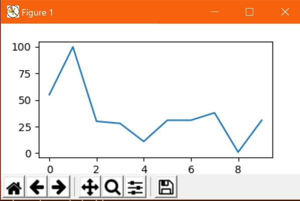
一番基本的なプロットをやってみる。
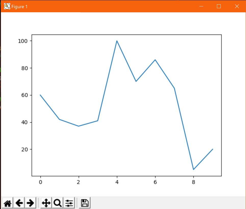
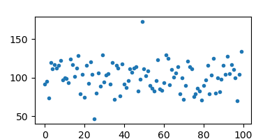
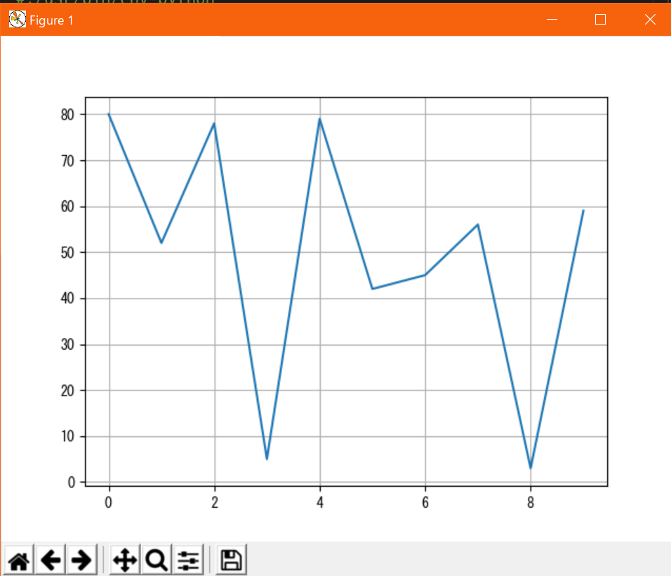
単一データfrom matplotlib import pyplot as plt from random import randint # データの定義(サンプルなのでテキトー) x = list(range(10)) y = [randint() for _ in x] # グラフの描画 plt.plot(x, y) plt.show()出力↓
とりあえず描画するだけならば非常にシンプルで、上記サンプルのように
matplotlibライブラリからpyplotモジュールをインポートし、リスト等で用意したデータをplt.plot()に渡すだけでよい。
plt.show()で出力例のようなウィンドウが開いて中にグラフが表示される。(注:サンプルのデータはランダムなのでグラフ自体は異なる)
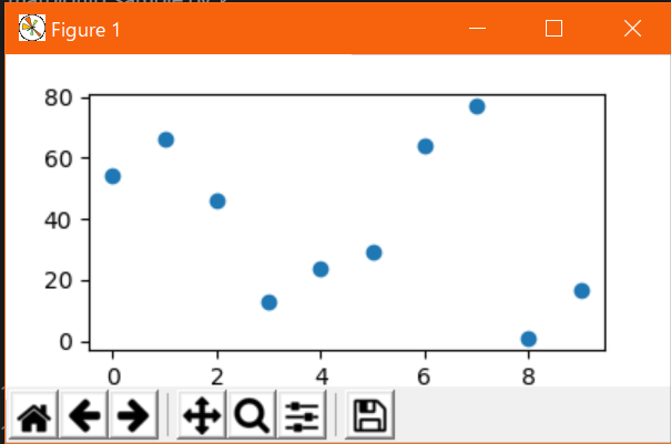
ちなみにpyplotモジュールはpltという名称に置換するのが慣例らしい。プロットしたいデータが複数ある場合は、
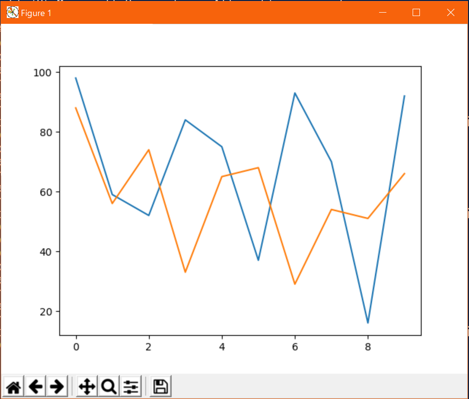
plt.plot()を描画したいデータ分だけ重ねればよい。複数のデータfrom matplotlib import pyplot as plt from random import randint # データの定義(サンプルなのでテキトー) x = list(range(10)) y1 = [randint(0, 100) for _ in x] y2 = [randint(0, 100) for _ in x] # グラフの描画 plt.plot(x, y1) plt.plot(x, y2) plt.show()出力↓
こんな感じに勝手に色分けされて描画される。
複数のグラフを1枚に描く
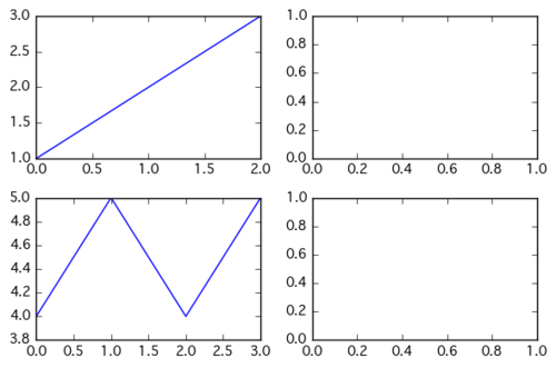
異なるデータを描画する際、重ねるのではなく別々に描画したいこともある。
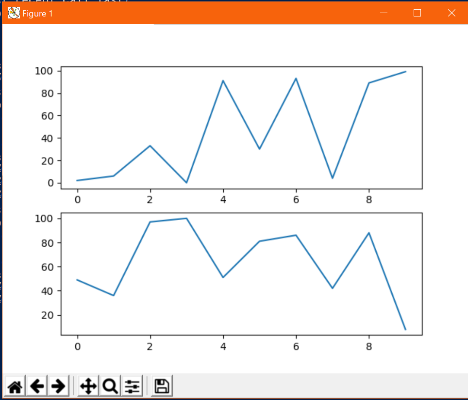
複数グラフfrom matplotlib import pyplot as plt from random import randint, random # データの定義(サンプルなのでテキトー) x = list(range(10)) y1 = [randint(0, 100) for _ in x] y2 = [randint(0, 100) for _ in x] # グラフの描画 fig = plt.figure() ax = fig.add_subplot(2, 1, 1) ax.plot(x, y1) ax = fig.add_subplot(2, 1, 2) ax.plot(x, y2) plt.show()出力↓
少し複雑になった。
最初に、fig = plt.figure()でグラフのインスタンスを取得し、ax = fig.add_subplot()でプロットエリアのインスタンスをaxに取得している。axに対してplotを実行することで異なるプロットエリアに描画している。
add_subplot()に渡す引数は左から、縦のプロットエリア数,横のプロットエリア数,割り当てるプロットエリア番号になっている。プロットエリア番号は左上から横⇒下の順で割りつく。2x2の場合の例
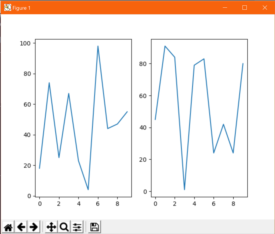
なので、サンプルのサブプロット部分の指定を下記のようにすると、横並びにもできる。
横並びax = fig.add_subplot(1, 2, 1) ax.plot(x, y1) ax = fig.add_subplot(1, 2, 2) ax.plot(x, y2)
ちなみに、サンプルでは
fig、axに明示的にプロットエリアのインスタンスを取得してからプロットしているが、下記のようにも書ける。少しラフな書き方# グラフの描画 plt.subplot(2, 1, 1) plt.plot(x, y1) plt.subplot(2, 1, 2) plt.plot(x, y2) plt.show()好みの問題かもしれないが、この記法で書いても劇的に短縮されるわけではないのでメリットは薄い。(気がする)
なお、
subplotでは強制的にグリッドレイアウトになるが、変則的なレイアウトにする手段もある。
ただし、大抵subplotで事足りる気がするのでこの記事には含まない。もし、必要になったらここの記事が参考になる。よく使うグラフの種類
ここまでの例ではすべて折れ線グラフを使っていたが、いろいろな種類のグラフを書くことができる。
折れ線グラフ:plot
plt.plot(x, y)
散布図:scatter
plt.scatter(x, y)
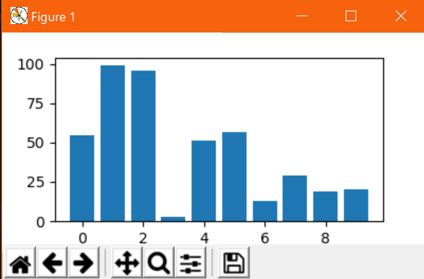
棒グラフ:bar
plt.bar(x, y)
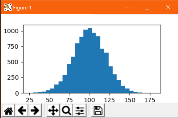
ヒストグラム:hist
plt.hist(y, 30)
ヒストグラム以外の種類は呼び出す関数を変えるだけで、x,yの指定通り描画できる。散布図は
plot関数でlinewidthとmarkerオプションを設定することでも作成できるが、scatter関数の場合は、関数名変えるだけなのでこちらのほうが楽。(scatterは厳密にはバブルチャート作成用らしい)
ヒストグラムに関してはランダムに存在するデータを第一引数に渡し、第二引数で分割数を指定する。上記のサンプルでは正規分布の10000件のデータをyに入れて、適当に30分割して表示してみた。
他にも円グラフやヒートマップなど色々あるが、ここではよく使うものだけまとめておく。ほかのグラフは公式ドキュメントに沢山の例があるので、描きたいグラフに近いものを参照すればよい。グラフの保存
ここまでの例では
plt.show()でグラフの表示をしてきた。これを使うと、pythonコード実行時にグラフ用のウィンドウが開いて中にグラフが表示される形になる。一応、このウィンドウから保存もできるが、連続で数枚のグラフを作る時や、画像サイズにこだわる時は一々表示はせずにグラフ画像の保存用関数plt.savefig("ファイル名.png")で保存できる。
ファイル形式は保存するファイル名末尾につけた形式で自動判別される。
上の図は適当な散布図をpng形式で保存したもの。
ファイル名にはパスを指定するので、imgディレクトリ等を先に作って、その中に連続で画像を保存とかもできる。保存先ディレクトリ自動作成を含んだコード例#!/usr/bin/env python # coding: utf-8 from matplotlib import pyplot as plt import numpy as np from pathlib import WindowsPath as Path # データの定義(サンプルなのでテキトー) x = range(100) y = np.random.normal(100, 20, 100) # 画像の保存先ディレクトリを作成 img_path = Path("./img") img_path.mkdir(exist_ok=True) # グラフの描画 plt.figure(figsize=(4, 2)) plt.plot(x, y, lw=0, marker='.') plt.savefig("./img/test.png")jupyterでの表示
jupyterのセルごとに実行結果をoutセルに表示できる。
%matplotlib inlineとノートブックの先頭などに書いておくだけで、他は通常通り書けばよい。
※いつからか不明だが、何も書かなくてもインライン表示できました。とりあえず実行して、表示できないときは上記を書くと解決するかもしれません。
markdown-preview-enhancedのコードチャンクでの表示
実験結果をレポートとしてまとめる時などに、markdown-preview-enhancedを使う場合、コードチャンクとして実行コードを埋め込むことができる。
通常、コードチャンクとしてpythonのコードを埋め込む時は、```python {cmd}
~
```のようにpython指定のコードブロックの後ろに
␣{cmd}をつける。
このままでmatplotlibの描画コードを実行すると、plt.show()で別ウィンドウが開いてしまう。
こんな感じ↓
そこで、コードブロックの後ろを
␣{cmd matplotlib}に変更すると、ドキュメント中に出力がインライン表示されるようになる。↓
hideも指定して、␣{cmd hide matplotlib}とすると、描画用のコードを隠してグラフだけ表示することもできる。※コードチャンク自体デフォルトではセキュリティ上offになっているので、公式ドキュメントの通り有効にしたときのみ使用できる。公式ドキュメントでも下記の注意書きがあるように、悪意あるコードを実行できてしまう危険があるので、機能の有効化は自己責任で。
⚠️ Script execution is off by default and needs to be explicitly enabled in Atom >package / VSCode extension preferences
Please use this feature with caution because it may put your security at risk! Your >machine can get hacked if someone makes you open a markdown with malicious code while >script execution is enabled.
Option name: enableScriptExecution
見た目の調整
ここまではデータをプロットするだけだったが、レポートに載せる時などは当然体裁を整えたくなる。
よく使うオプション
軸、目盛り関連
軸範囲の調整:xlim, ylim
表示する軸範囲をを設定するオプション。
x軸はplt.xlim(min, max)、y軸はplt.ylim(min, max)にそれぞれ上下限値を指定する。
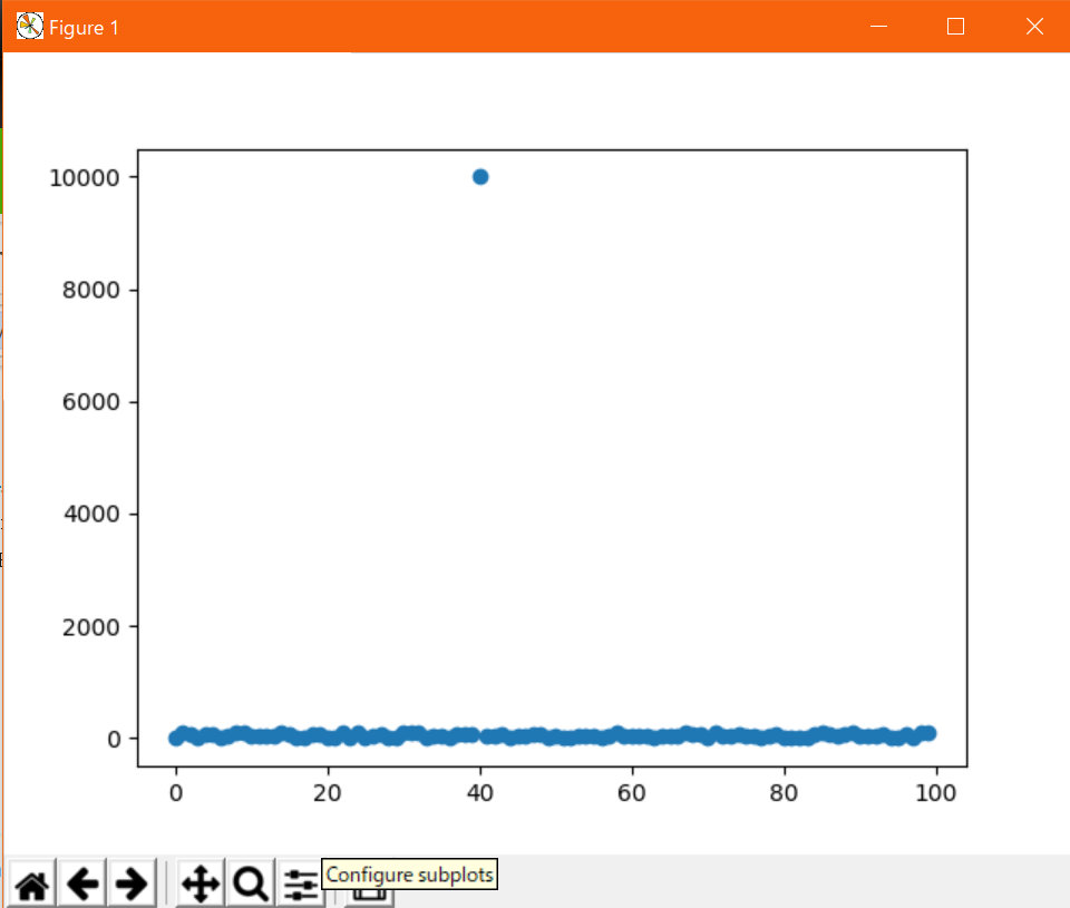
なお、axesを使う場合はax.set_xlim(min, max)とax.set_ylim(min, max)と若干名称が変化する。例えば、下記コードは散布図を描画するが、基本0~100のデータ分布中に10000の値が紛れさせている。
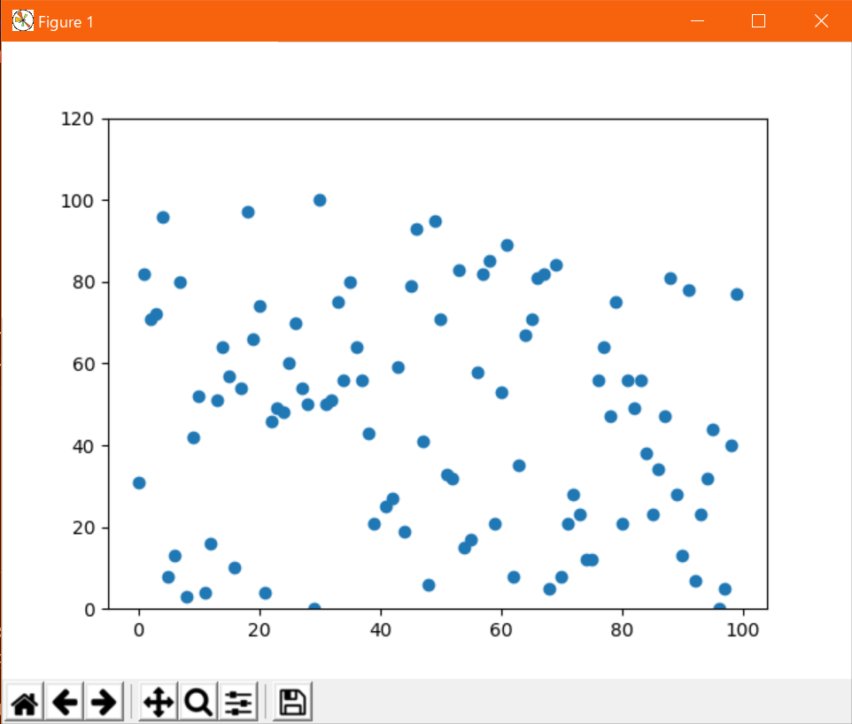
#!/usr/bin/env python
# coding: utf-8
from matplotlib import pyplot as plt
import random

# データの定義(サンプルなのでテキトー)
x = range(100)
y = [random.randint(0, 100) for _ in range(40)]
y.append(10000)
y.extend([random.randint(0, 100) for _ in range(59)])

# グラフの描画
plt.scatter(x, y)
plt.show()
これを描画するとこうなる。
こんな外れデータを無視して分布が集中しているところを見たくなったりするときに、データから外れ値を除く処理を掛けなくても、y軸の描画範囲を絞るだけで見れるようになる。
y軸描画範囲を0~120に制限#!/usr/bin/env python # coding: utf-8 from matplotlib import pyplot as plt import random # データの定義(サンプルなのでテキトー) x = range(100) y = [random.randint(0, 100) for _ in range(40)] y.append(10000) y.extend([random.randint(0, 100) for _ in range(59)]) # グラフの描画 plt.scatter(x, y) plt.ylim(0, 120) plt.show()
数値でない軸目盛りを使う
x軸には時折数値でない値を使いたいこともある。
文字列をそのまま軸目盛りに使いたい場合
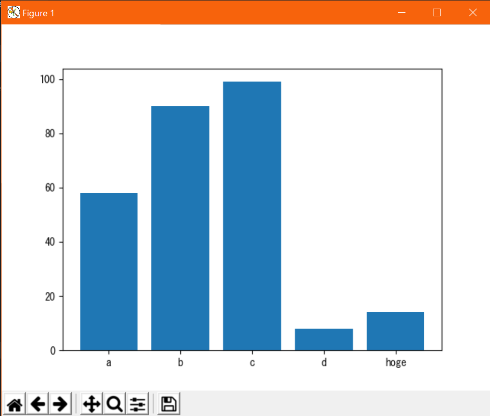
項目ごとに正規化した値を比較するようなグラフとかの場合は、x軸に項目名の文字列リストを指定するだけで自動的に項目名を軸にしてくれる。
例#!/usr/bin/env python # coding: utf-8 from matplotlib import pyplot as plt import random # データの定義(サンプルなのでテキトー) x = ['a', 'b', 'c', 'd', "hoge"] y = [random.randint(0, 100) for _ in x] # グラフの描画 plt.bar(x, y) plt.show()出力↓
プロットは値そのままで、描画上文字列に置換したい場合
任意の文字列を目盛りに振りたい時は、x軸は
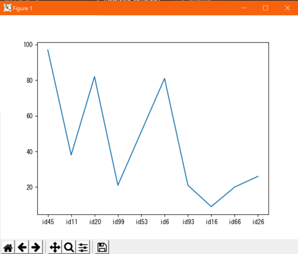
plt.xticks(x, ticks)、y軸はplt.yticks(y, ticks)を使う。x,yは目盛り値のリスト、ticksには目盛りに対応するラベル(文字列とか)のリストを渡す。ticksを省略すると目盛りの値がそのままラベルになる。
なお、axesに設定する場合はset_xticks(),set_yticks()になる。x軸の値ラベルを適当な文字列で置換する例#!/usr/bin/env python # coding: utf-8 from matplotlib import pyplot as plt import random # データの定義(サンプルなのでテキトー) x = range(10) xticks = ["id{}".format(x) for x in random.sample(range(100), len(x))] y = [random.randint(0, 100) for _ in x] # グラフの描画 plt.plot(x, y) plt.xticks(x, xticks) plt.show()出力↓
また、
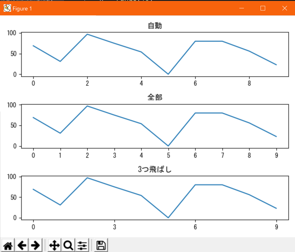
xticks,yticksは軸の目盛りを調整するものになるので、デフォルトの目盛り間隔が広すぎる/狭すぎるといったときに、任意の間隔に調整するのにも使う。目盛り間隔による違い#!/usr/bin/env python # coding: utf-8 from matplotlib import pyplot as plt import random # データの定義(サンプルなのでテキトー) x = range(10) xticks = ["id{}".format(x) for x in random.sample(range(100), len(x))] y = [random.randint(0, 100) for _ in x] # グラフの描画 fig = plt.figure() ax = fig.add_subplot(3, 1, 1) ax.plot(x, y) ax.set_title("自動") ax = fig.add_subplot(3, 1, 2) ax.plot(x, y) ax.set_xticks(x) ax.set_title("全部") ax = fig.add_subplot(3, 1, 3) ax.plot(x, y) ax.set_xticks([i for i in x[::3]]) ax.set_title("3つ飛ばし") plt.tight_layout() plt.show()出力↓
軸目盛を表示したくない場合
plt.xticks([])のように空のリストを渡せば軸目盛を消せる。
なお、axesに設定する場合はset_xticks(),set_yticks()になる。
グリッドの表示/非表示
グラフによってはグリッド線のガイドがあると見やすくなるものがある。グリッドは
plt.grid()で表示できる。グリッド線表示例#!/usr/bin/env python # coding: utf-8 from matplotlib import pyplot as plt import random # データの定義(サンプルなのでテキトー) x = range(10) y = [random.randint(0, 100) for _ in x] # グラフの描画 plt.plot(x, y) plt.grid() plt.show()出力↓
オプション引数で
axis=に"x"や"y"を指定すると、指定した側だけグリッド線を表示できる。
データの表示関連
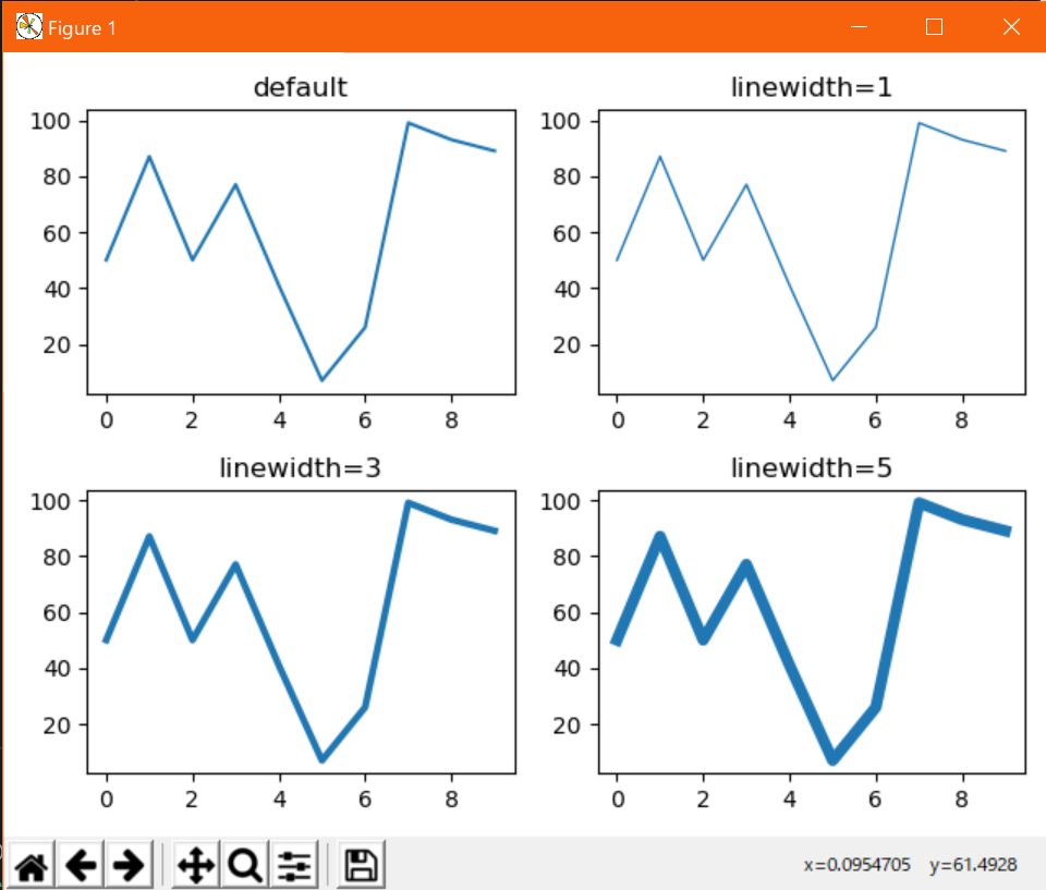
線の幅を調整:linewidth
折れ線で接続する線の幅を調整するオプション。
plt.plot(x, y, linewidth=xx)または、plt.plot(x, y, lw=xx)と指定する。(xxは任意の値)表示例↓
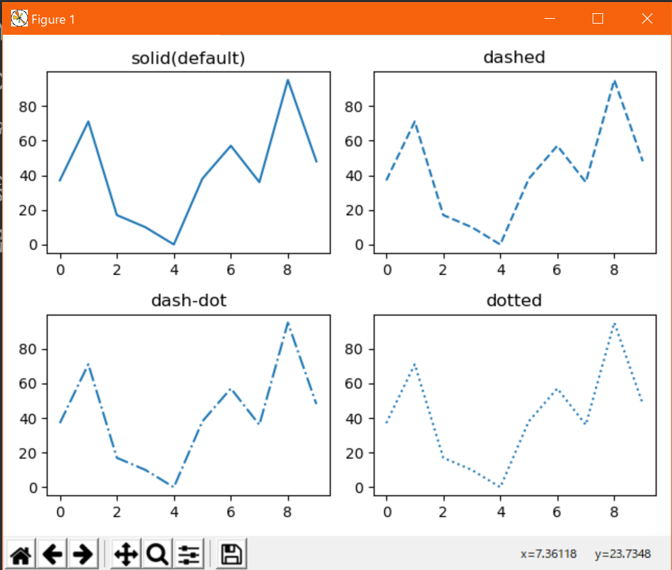
線の種類:linestyle
折れ線で接続する線の種類を調整するオプション。
plt.plot(x, y, linestyle=xx)または、plt.plot(x, y, ls=xx)と指定する。(xxは任意の指定子)
指定子 種類 "-" 実線 "--" 破線 "-." 一点鎖線 ":" 点線 表示例↓
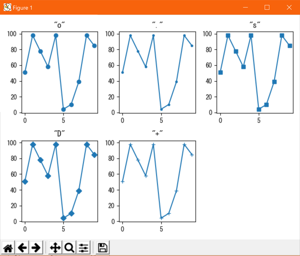
点の種類:marker
プロットする点の種類を調整するオプション。
plt.plot(x, y, marker=xx)と指定する(xxは任意の指定子)
指定子は大量にあるが、主に使うものをピックアップしたのが下表。全種確認したい時は公式ドキュメントを参照。
指定子 種類 "o" 丸 "." 点 "s" 四角 "D" ダイヤ "+" プラス 表示例↓
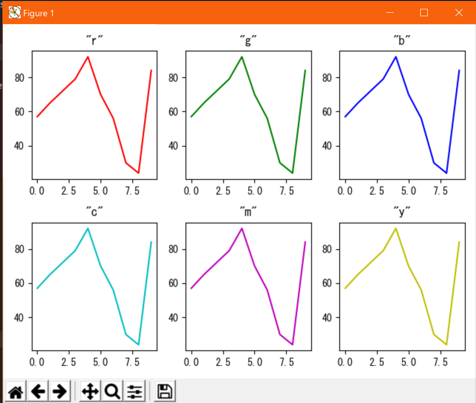
線、点の色:color
描画する線及び点の色を調整するオプション。
plt.plot(x, y, color=xx)またはplt.plot(x, y, c=xx)と指定する(xxは任意の色名)
指定する色名の内、下表の色は短縮指定子を使える。
下表に無い色でもかなりの色がプリセットとして色名指定できるようになっている。詳しくは公式ドキュメント参照。
指定子 色 フルネーム 'r' 赤 "red" 'g' 緑 "green" 'b' 青 "blue" 'c' シアン "cyan" 'm' マゼンタ "magenta" 'y' 黄 "yellow" 'k' 黒 "black" 'w' 白 "white" 表示例↓
その他
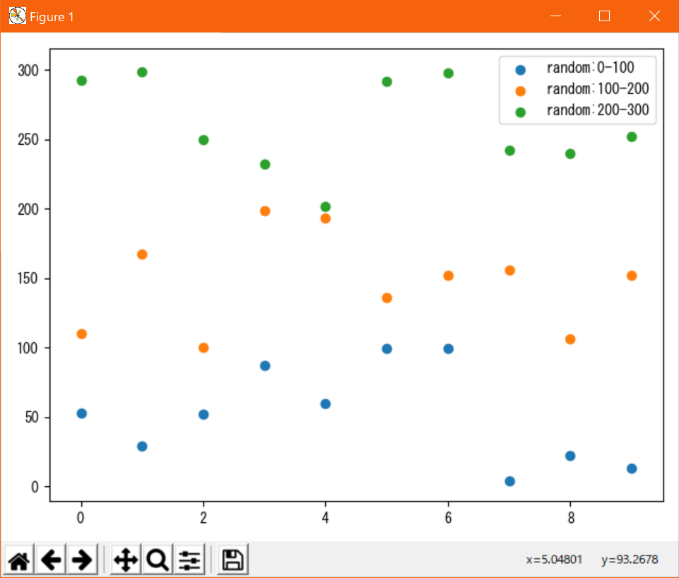
凡例の表示
プロットしたデータの凡例を表示する機能。
表示例↓
表示例のコード#!/usr/bin/env python # coding: utf-8 from matplotlib import pyplot as plt import random # データの定義(サンプルなのでテキトー) x = range(10) fig, ax = plt.subplots(1, 1) for i in range(3): lower = 100 * i upper = lower + 100 y = [random.randint(lower, upper) for _ in x] ax.scatter(x, y, label="random:{}-{}".format(lower, upper)) plt.legend() plt.tight_layout() plt.show()なお、凡例の表示位置を
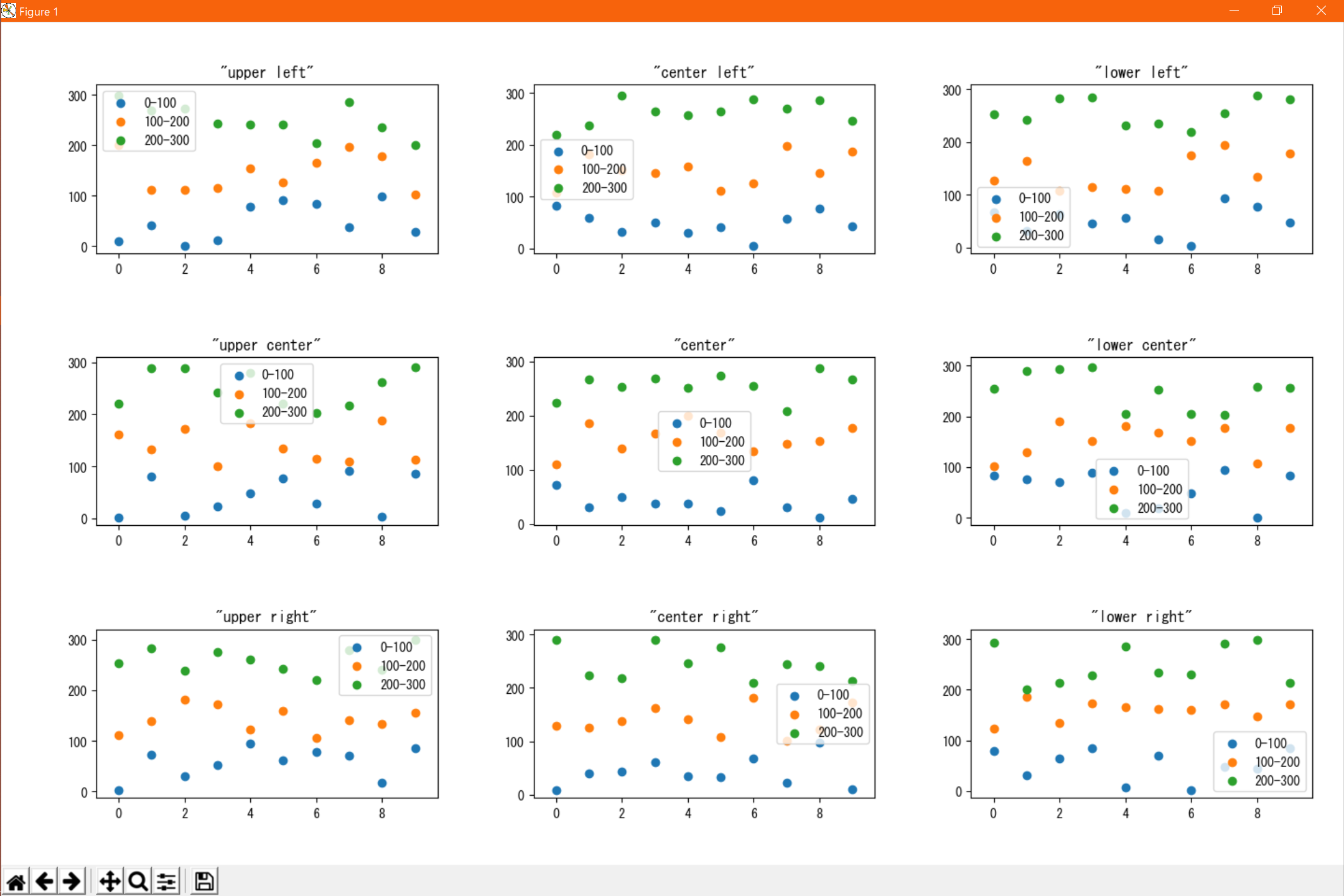
plt.legend(loc=xx)で指定できる。(xxは任意のパターンの指定子)
なお、axesの場合も同じメソッド名でよい。
指定パターンは下表の通り。
指定子 位置 "best" 自動(標準) "upper left" 左上 "center left" 左中央 "lower left" 左下 "upper center" 中央上 "center" 中央 "lower center" 中央下 "upper right" 右上 "center right" 右中央 "lower right" 右下 表示例↓
表示例のコード#!/usr/bin/env python # coding: utf-8 from matplotlib import pyplot as plt import random # データの定義(サンプルなのでテキトー) x = range(10) # グラフの描画 fig = plt.figure() locs = [ "{} {}".format(a, b) for b in ["left", "center", "right"] for a in ["upper", "center", "lower"] if not (a == "center" and b == "center") ] locs.insert(len(locs) // 2, "center") for j, loc in enumerate(locs, 1): for i in range(3): lower = 100 * i upper = lower + 100 y = [random.randint(lower, upper) for _ in x] ax = fig.add_subplot(3, 3, j) ax.scatter(x, y, label="{}-{}".format(lower, upper)) ax.set_title("\"{}\"".format(loc)) ax.legend(loc=loc) plt.tight_layout() plt.show()グラフタイトルの表示
グラフに任意のタイトルを書く機能。
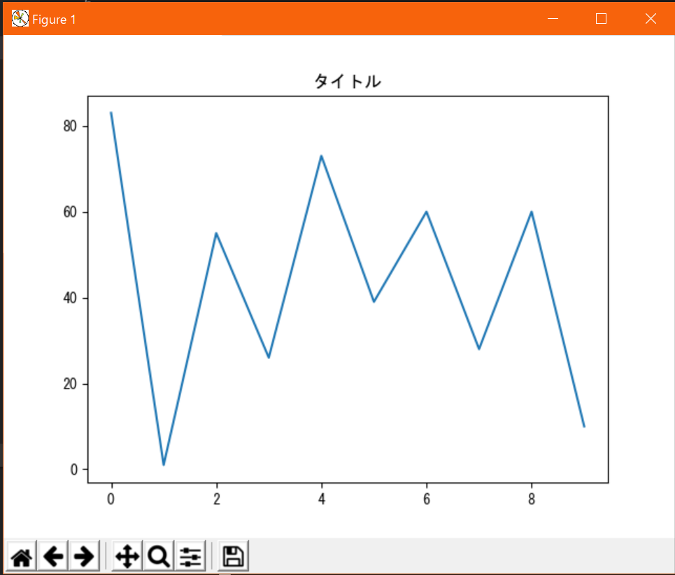
plt.title(xx)で指定する。(xxは表示したい任意の文字列)なお、axesの場合はax.set_title(xx)となる。表示例↓
表示例のコード#!/usr/bin/env python # coding: utf-8 from matplotlib import pyplot as plt import random # データの定義(サンプルなのでテキトー) x = range(10) y = [random.randint(0, 100) for _ in x] # グラフの描画 plt.plot(x, y) plt.title("タイトル") plt.show()任意のテキストの表示
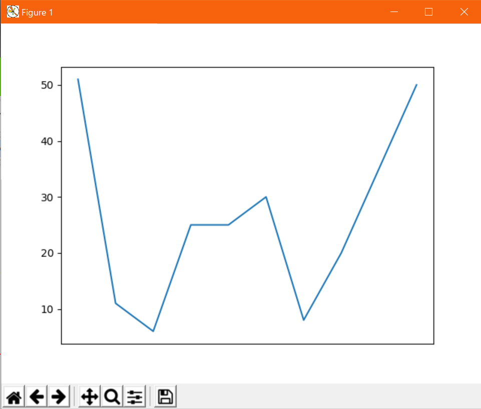
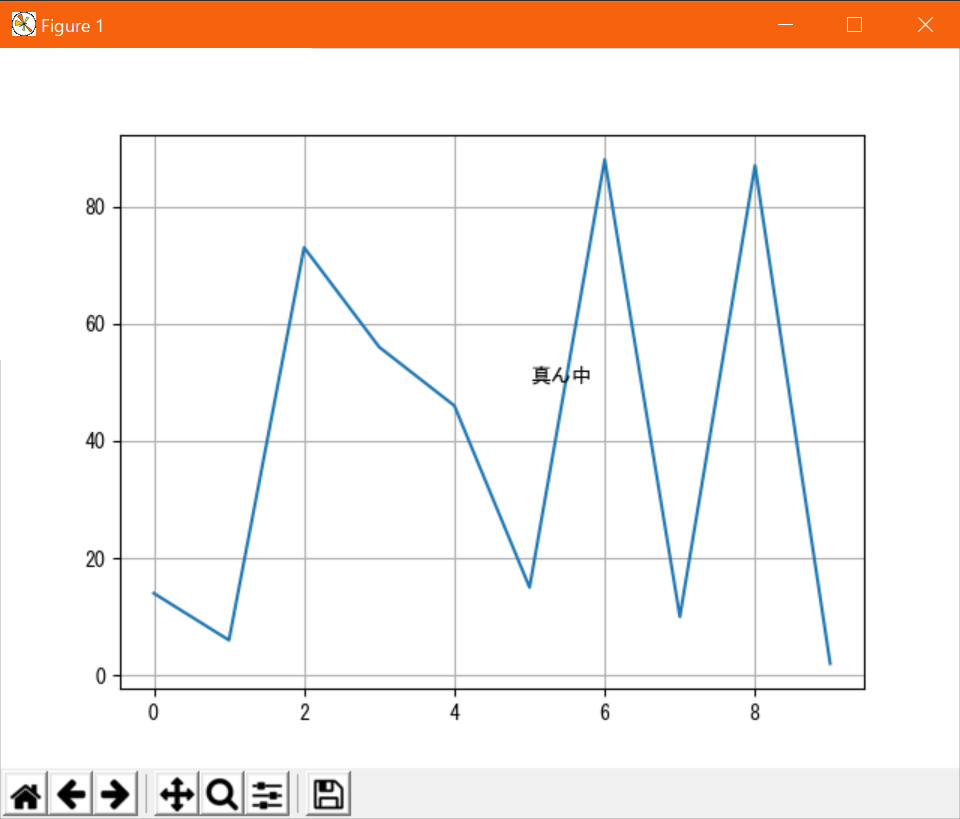
axes内の任意座標を指定して、指定したテキストを描画する機能。
plt.text(x, y, s)で指定する。表示例↓
表示例のコード#!/usr/bin/env python # coding: utf-8 from matplotlib import pyplot as plt import random # データの定義(サンプルなのでテキトー) x = range(10) y = [random.randint(0, 100) for _ in x] # グラフの描画 plt.plot(x, y) plt.text(5, 50, "真ん中") plt.grid() plt.show()終わりに
普段よく使う機能をまとめてみたが、かなりのボリュームになってしまった…
matplotlibにはまだまだ使ったことない機能も沢山あるが、次はアニメーションをまとめたいと思います。参考


- 投稿日:2019-07-07T20:15:47+09:00
matplotlibの描画の基本 - figやらaxesやらがよくわからなくなった人向け
matplotlibは、figureやsubplotなどなどがどう働いているのかが分かりにくい。
そこで、ここでは、matplotlibの描画の構造について説明する。これ以降、matplotlib.pyplotをpltとしてimportしているとする。
import matplotlib.pyplot as pltplt.figure()
plt.figure()が最初に出てくることが多い。figure()はFigureインスタンスを作成する。
Figureインスタンスは、描画全体の領域を確保する。
引数では以下を指定できる。
- figsize: (width, height)のタプルを渡す。単位はインチ。
- dpi: 1インチあたりのドット数。
- facecolor: 背景色
- edgecolor: 枠線の色
plt.figure()では描画領域の確保だけなので、グラフは何も描画されない。
fig.add_subplot()
plt.figure()にグラフを描画するためにsubplotを追加する必要がある。
subplotの追加は、add_subplotメソッドを使用する。fig = plt.figure() fig.add_subplot(111)これで以下のように軸などのグラフの描画領域が追加される。
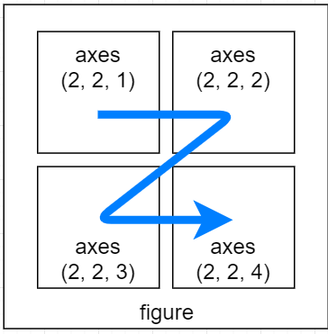
111の意味は、1行目1列の1番目という意味で、subplot(1,1,1)でも同じである。
subplotはAxesオブジェクトを返す。
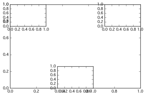
Axesは、グラフの描画、軸のメモリ、ラベルの設定などを請け負う。add_subplotは基本的に上書きとなる。以下は、どういう構成化わかりすくするために、わざと上書きしたもの。
fig = plt.figure()
fig.add_subplot(1, 1, 1)
fig.add_subplot(3, 3, 1)   # 3x3の1つめ(左上)
fig.add_subplot(3, 3, 3)   # 3x3の3つめ(右上)
fig.add_subplot(3, 3, 8)   # 3x3の8つめ(真ん中下)
plt.subplot()
plt.subplot()はadd_subplotと同様に、引数に行数列数及び何番目かを指定できる。
add_subplotとの違いは、現在の描画領域(fig = figure()のこと)に追加するメソッドであるということ。
あまりないと思うが、figure()を何個も立ち上げてるときに、どれを操作しているかわかりにくくなる。plt.subplot(3,3,1) plt.subplot(3,3,3) plt.subplot(3,3,5) plt.subplot(3,3,9)
subplotはsubplot以前に描画していたfigureとかぶった場合、前のfigureを消す性質を持っている。
plt.plot([1,2,3])
plt.subplot(211)   # このタイミングで plt.plot([1,2,3]) は消されてしまう。
plt.plot(range(12))
plt.subplot(212)
plt.subplots()
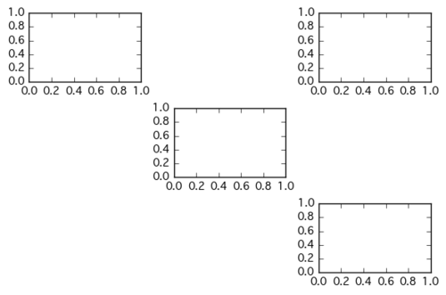
plt.subplot()と似たものとしてplt.subplots()もある。
返り値はfigとAxesまたはAxesオブジェクトの配列。plt.subplots()は実は、fig = figure()をした後、fig.add_subplot(111)した場合と同じである。
subplots()も、add_subplotの場合と同様にAxesオブジェクトを返す。fig = plt.figure() plt.add_subplot(111)plt.subplots()の引数に行数列数を与えることで、複数のAxesオブジェクトを生成できる。
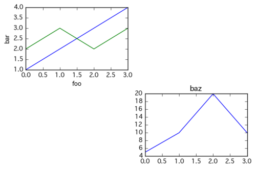
fig, axes= plt.subplots(2,2)   # axesはAxesオブジェクトの2x2の配列
axes[0][0].plot([1,2,3])
axes[1][0].plot([4,5,4,5])
上記スクリプトの出力結果は以下のようになる。
Axes
Axesオブジェクトは、実際のデータの描画の役割を持っている。
Axesオブジェクトに対して描画するデータを与えたり、set_xlabel、set_ylabel、set_titleで
ラベルやタイトルの設定をできる。
また、同じAxesオブジェクトにplotを重ねることもできる。ax1 = plt.subplot(2,2,1) # 4x4の1番目 ax4 = plt.subplot(2,2,4) # 4x4の4番目 ax1.plot([1,2,3,4]) # 1番目に描画 ax1.plot([2,3,2,3]) # 1番目に追加描画 ax1.set_xlabel('foo') # 1番目にxラベルを追加 ax1.set_ylabel('bar') # 1番目にyラベルを追加 ax4.plot([5,10,20,10]) # 4番目に描画 ax4.set_title('baz') # 4番目にタイトルを追加
plt.title()、plt.xlabel()、plt.ylabel()
グラフを1つずつ描画しているときは、plt.title()、plt.xlabel()、plt.ylabel()をよく使うのだが、
結局これは何かというと、ax = subplot(111)にたいして、ax.set_title()、ax.set_xlabel()、ax.set_ylabel()
とやっていることと同じとなる。plt.gcf()
figureをたくさん立ち上げているとどのfigureにいるかわからなくなることがある。
現在のfigureを確認するためにはplt.gcf()を使う。gcfはget current figureの略。
以下の例ではそれぞれplt.gcf()の出力結果が変わることが分かる。fig1 = plt.figure() print(plt.gcf().number) # => 1 fig2 = plt.figure() print(plt.gcf().number) # => 2 plt.close() print(plt.gcf().number) # => 1plt.gca()
plt.gcf()と似た関数でplt.gca()がある。
これは、現在のAxesオブジェクトを返す。
ax = subplot(111)でやらずにあとからAxesオブジェクトを変数に定義できる。plt.subplot(111) ax = plt.gca()

- 投稿日:2019-07-07T20:14:45+09:00
因果推論でデジタル広告のCPA・ROASを改善する方法
記事の概要
現在、デジタル広告の成長率は著しい。インターネットに接続すると、
多くのページに広告が埋め込まれている。広告には必ず配信している
広告主がおり、多額の広告費用が使われている。しかし、多くの広告主は費用を下げたいと考えているはずだ。
よって、今回はコンバージョン数を下げずに広告費を減らせる
可能性がある方法を記載する。広告主が取り扱う広告のKPI
広告主は主に以下の指標でデジタル広告を評価する。
CVs = 訪問ユーザ数(全部) x コンバージョン率
Cost = 訪問ユーザ数(広告経由) x クリック単価
Revenue = 訪問ユーザ数(全部) x コンバージョン率 x 単価 x 購入回数
CPA = Cost / Cvs
ROAS = Revenue / Cost訪問ユーザ数(広告経由) x クリック単価が広告費用となる。
これを下げれば、CPA・ROASも改善する仕組みだ。広告の貢献度の評価
広告の分析にはアトリビューションというものがあり、広告の貢献度を図るために定義された指標だ。
購入の直前に触れた広告のみを評価するラストクリックや、購入までの最初に触れた広告のみを評価する
ファーストクリックが一般的だ。
https://anagrams.jp/blog/basic-of-attribution/アトリビューション分析によって広告媒体のCPAやROASを計測し、どの時点で貢献しているかが可視化できる。
ただ、これだけでは広告の貢献度を図るのは難しい。なぜなら、広告に触れた
ユーザがコンバージョンしても、広告がきっかけなのかはわからない。
つまり、「広告に触れなくても」コンバージョンしていた可能性がある。因果推論によるターゲット分類
ここで使用するのが因果推論だ。因果推論は簡潔に言うと「原因」と
「結果」を明らかにする手法だ。例えば医療業界で言うと、「この薬を
飲んだから(原因)、病気が治った(結果)」、ということを検証するために
利用される。以下の事例がわかりやすい。
https://healthpolicyhealthecon.com/2014/09/30/study-design-overview/広告で言うと「広告に触れて(原因)、商品を購入した(結果)」と
置き換えられる。因果推論を使用する場合、「ある広告に触れたユーザ」と
「ある広告に触れなかったユーザ」が、それぞれ「コンバージョンしたか否か」
のデータを収集する。このデータを因果推論のモデルに学習させ、テストデータで予測させると、
ターゲットを以下のように分類できる。① あまのじゃくユーザ:広告を配信すると、コンバージョンしなくなる。
② 無関心ユーザ:広告を配信有無に関わらず、コンバージョンしない。
③ 確実購入ユーザ:広告を配信有無に関わらず、コンバージョンする。
④ 説得可能ユーザ:広告を配信すると、コンバージョンする。例えば、モデルの予測で④の数が多ければ、広告がユーザを説得して
いることになるので、それは配信するべき広告となる。しかし、①②③の数が多い場合は広告を配信しなくてもユーザは
コンバージョンするし、コンバージョンを阻害している可能性もある。CPA・ROASを改善するために
ここまででわかる通り、因果推論でCPA・ROASを改善する方法は以下だ。
・因果推論モデルを用いてターゲットを分類する。
・説得可能ユーザが多い広告の出稿を増やすか、配信不要ユーザが多い広告の
出稿を減らす。この流れをPythonで実装してみる。
1. モジュールインポート
# Main imports
from econml.metalearners import TLearner, SLearner, XLearner, DomainAdaptationLearner, DoublyRobustLearner
from sklearn.linear_model import LinearRegression
from sklearn.ensemble import RandomForestRegressor, RandomForestClassifier, GradientBoostingRegressor
from sklearn.model_selection import train_test_split

# Helper imports
import os, sys
import numpy as np
import pandas as pd
from numpy.random import binomial, multivariate_normal, normal, uniform
import matplotlib.pyplot as plt
2.データセットの作成
データは以下から取得。BigQueryに存在するGoogleAnalyticsの
公開データセットで、サイトへのアクセス情報だけでなく広告経由の流入も
格納されている。既にダウンロードして、results_bqga.csvにまとめている。
https://bigquery.cloud.google.com/table/bigquery-public-data:google_analytics_sample.ga_sessions_20170801os.listdir("../input") df_bqga = pd.read_csv("../input/results_bqga.csv") # 欠損値の確認 df_bqga.isnull().sum() total_visits 0 total_transaction 890508 campaign 0 source 0 medium 0 fullVisitorId 0 visitNumber 0 # 欠損値を0に変換 df_bqga["total_transaction"] = df_bqga["total_transaction"].apply(lambda x : 0 if x != x else x) # ユーザ、参照元、流入経路、キャンペーンでグルーピング cols = ["fullVisitorId", "source", "medium", "campaign", "visitNumber", "total_visits"] df_bqga_grp = df_bqga.groupby(by=cols).sum().reset_index()3. CATE計算のためのデータ作成
CATEは「ある特徴量で条件付けた際の介入の因果効果の期待値」と言える。
つまりCATEが高いユーザは広告を付与した場合の効果が高いので、広告を配信するべきという結論が得られる。主に3つのデータが必要である。・Outcome(Y) = 目的変数でコンバージョンを達成したか、売上高など
・Treatment(T) = 広告やクーポンなど、アクションに触れたか否か
・Feature(X)= サイト訪問数や属性など、ユーザの特徴以下のコードで上記のデータを作成している。
# Treatmentの作成(広告に触れたか否か)
df_bqga_grp["Treatment"] = df_bqga_grp.medium.apply(lambda x : 1 if x in ["cpc", "cpm", "affiliate"] else 0)

# Outcomeの作成(購入したか否か)
df_bqga_grp["Outcome"] = df_bqga_grp.total_transaction.apply(lambda x : 0 if x == 0 else 1)

# Featureの作成(自然検索で訪問したか、再訪問したか、何回訪問したか)
df_bqga_grp["is_organic"] = df_bqga_grp.medium.apply(lambda x : 1 if x == "organic" else 0)
df_bqga_grp["is_return"] = df_bqga_grp.visitNumber.apply(lambda x : 0 if x == 1 else 1)
df_bqga_grp = pd.get_dummies(data=df_bqga_grp, columns=["total_visits"])

# 不要な列の作成
df_bqga_grp.drop(columns=["source", "medium", "campaign", "visitNumber" ,"total_transaction"], axis=1, inplace=True)

df_data = df_bqga_grp.groupby(by=["fullVisitorId"]).sum().reset_index()

# 全データを0 or 1に変換
df_data.iloc[:, 1] = df_data.iloc[:, 1].apply(lambda x : 0 if x == 0 else 1)
df_data.iloc[:, 2] = df_data.iloc[:, 2].apply(lambda x : 0 if x == 0 else 1)
df_data.iloc[:, 3] = df_data.iloc[:, 3].apply(lambda x : 0 if x == 0 else 1)
df_data.iloc[:, 4] = df_data.iloc[:, 4].apply(lambda x : 0 if x == 0 else 1)
df_data.iloc[:, 5] = df_data.iloc[:, 5].apply(lambda x : 0 if x == 0 else 1)
df_data.iloc[:, 6] = df_data.iloc[:, 6].apply(lambda x : 0 if x == 0 else 1)
df_data.iloc[:, 7] = df_data.iloc[:, 7].apply(lambda x : 0 if x == 0 else 1)

# 不均衡データの修正
df_case1 = df_data[(df_data["Treatment"] == 1) & (df_data["Outcome"] == 1)]
df_case2 = df_data[(df_data["Treatment"] == 1) & (df_data["Outcome"] == 0)].iloc[0:1000, :]
df_case3 = df_data[(df_data["Treatment"] == 0) & (df_data["Outcome"] == 1)].iloc[0:1000, :]
df_case4 = df_data[(df_data["Treatment"] == 0) & (df_data["Outcome"] == 0)].iloc[0:1000, :]
4. データ分割
トレーニング&テストデータに分割
train_df, test_df = train_test_split(df_data, test_size=0.2, random_state=0, stratify=df_data['Treatment'])

# ユーザIDを抽出しておき、データセットからはユーザIDを削除
user_ids = test_df.fullVisitorId
train_df.drop(["fullVisitorId"], inplace=True, axis=1)
test_df.drop(["fullVisitorId"], inplace=True, axis=1)
5. CATEの計算と予測(ここからが本題)
先ほど作成したデータから広告を配信するべきユーザ=CATE値が高い
ユーザを算出する。今回はeconmlを用いて実行する。
モジュールの詳細を知りたい方は以下を参照してほしい。
https://github.com/microsoft/EconMLEconMLとは?
EconMLはMicrosoftが作成したパッケージで、計量経済学と機械学習を
融合させたもの。このツールを用いて、意思決定を自動化することが
最終目的らしい。今回はEconMLを用いてユーザ毎のCATE値を計算してみる。データの投入
# 学習に必要なデータを投入
T = train_df.Treatment
Y = train_df.Outcome
X = train_df.drop(["Outcome", "Treatment"], axis=1)

# テスト用データにはユーザの特徴のみを投入しておく
X_test = test_df.drop(["Outcome", "Treatment"], axis=1)
モデル学習
EconMLには様々な計算用アルゴリズムが用意されている。その中の一つで
Meta-Learnersパッケージの中からDR-Learnerのアルゴリズムを使用して
学習する。# Instantiate Doubly Robust Learner outcome_model = GradientBoostingRegressor(n_estimators=100, max_depth=6) pseudo_treatment_model = GradientBoostingRegressor(n_estimators=100, max_depth=6) propensity_model = RandomForestClassifier(n_estimators=100, max_depth=6, class_weight='balanced_subsample') DR_learner = DoublyRobustLearner(outcome_model=outcome_model, pseudo_treatment_model=pseudo_treatment_model, propensity_model=propensity_model) # Train DR_learner DR_learner.fit(Y, T, X)CATE値の予測
最後にEconMLでCATE値を予測して、ユーザIDと並べてみる。
# Estimate treatment effects on test data
DR_te = DR_learner.effect(X_test)
df_cate = pd.DataFrame({"user-id" : user_ids, "cate" : DR_te})
df_cate.head()
    user-id         cate
    2.121750e+15    -0.188887
    2.766490e+17    -0.086540
    2.252240e+15    -0.137244
    1.563470e+15    -0.188887
    1.677000e+15    0.597261
CATEを計算した後
これでユーザ毎のCATE値が計算できた。あとはこの値に従って広告を配信する
ユーザと停止するユーザを振り分ける。ただ、いきなり広告配信を取りやめる
のは勇気がいるので、徐々に予算を減らしていき総コンバージョン数が
変わらないことを検証しながら運用していくのだ。機械学習はマーケティングの分野にも確実に応用されていき、クリエイティブ
出ない分野はどんどん効率化されていくだろう。
- 投稿日:2019-07-07T19:21:30+09:00
Pythonで小数を取り扱う話
はじめに
Pythonで、というかコンピュータは小数の扱いが苦手です。
というのもコンピュータは2進数を基準に計算しており、小数を取り扱うのが難しいからです。多くの場合、コンピュータは小数を扱うとき、その値の近似値を表します。
そのため、次のような計算を行うと、正確な数を計算することができません。
A = 0.33
B = 10.0
print("ans: " + str(A * B))

# ans: 3.3000000000000003
これはつまり、次のような事に注意が必要という事です。
A = 0.33
B = 10.0

if(A * B == 3.3):
    print("一致")
else:
    print("不一致")

# 不一致
というわけでpythonで小数を取り扱うようなライブラリを調べてみました。
decimal
decimalはpythonの標準ライブラリです。
10進数の浮動小数点のための計算を行うために設計されています。この型を使用すると、人間の感覚に近い計算が行えます。
Doc: https://docs.python.org/ja/3/library/decimal.html
from decimal import *

x = Decimal("0.33")
x10 = x * 10

print("ans: " + str(x10))
print("type: " + str(type(x10)))

# ans: 3.30
# type: <class 'decimal.Decimal'>
Decimal型の変数はintとの計算では明示的にキャストする必要はありません。
x2 = x + 1
print(x2)

# 1.33
だたしfloat型は明示的にキャストをする必要があります。
x2 = x + 0.003
print(x2)

# TypeError: unsupported operand type(s) for +: 'decimal.Decimal' and 'float'

x2 = x + Decimal(0.003)
print(x2)

# 0.3330000000000000000624500451
あれ?
float型からDecimal型へのキャストは注意が必要
float型からDecimal型にキャストすると、うまく動作しないようです。
float型は小数の近似値をDecimal型に渡すので、その近似値を正確にDecimal型が読んでしまため、このような処理になったものと思われます。
なので、この場合はstr型を経由して、Decimal型にキャストすると良いでしょう。print(Decimal(0.003)) # 0.003000000000000000062450045135165055398829281330108642578125 print(Decimal(str(0.003))) # 0.003終わりに
冒頭で失敗していた比較の演算は次のようになります。
A = Decimal(str(0.33))
B = Decimal(str(10.0))

if(float(A * B) == 3.3):
    print("一致")
else:
    print("不一致")

# 一致
- 投稿日:2019-07-07T19:04:26+09:00
【Tensorflow・VGG16】転移学習による画像分類
やること(概要)
- 1. 画像データの収集
- 2. データセットの作成(画像データの変換)
- 3. モデルの作成 & 学習
- 4. 実行(コマンドライン)
動作環境
- macOS Catalina 10.15 beta
- Python 3.6.8
- flickapi 2.4
- pillow 6.0.0
- scikit-learn 0.20.3
- google colaboratory
実施手順
1. 画像データの収集
・3種類(りんご、トマト、いちご)の画像分類を実施するため、画像ファイルをflickrから取得
・flickrによる画像ファイルの取得方法は前回記事で書いたこちら
・それぞれ300枚の画像ファイルを取得
・検索キーワードは、「apple」、「tomato」、「strawberry」を指定
・flickrからダウンロードした不要なデータ(検索キーワードと関係ない画像ファイル)は目で見て除外しておくdownload.pyfrom flickrapi import FlickrAPI from urllib.request import urlretrieve import os, time, sys # Set your own API Key and Secret Key key = "XXXXXXXXXX" secret = "XXXXXXXXXX" wait_time = 0.5 keyword = sys.argv[1] savedir = "./data/" + keyword flickr = FlickrAPI(key, secret, format='parsed-json') result = flickr.photos.search( text = keyword, per_page = 300, media = 'photos', sort = 'relevance', safe_search = 1, extras = 'url_q, license' ) photos = result['photos'] for i, photo in enumerate(photos['photo']): url_q = photo['url_q'] filepath = savedir + '/' + photo['id'] + '.jpg' if os.path.exists(filepath): continue urlretrieve(url_q,filepath) time.sleep(wait_time)2. データセットの作成(画像データの変換)
・取得した画像ファイルをnumpy形式(バイナリファイル -> .npy)で保存
・VGG16のデフォルトサイズの224にresizegenerate_data.pyfrom PIL import Image import os, glob import numpy as np from sklearn import model_selection classes = ['apple', 'tomato', 'strawberry'] num_classes = len(classes) IMAGE_SIZE = 224 # Specified size of VGG16 Default input size in VGG16 X = [] # image file Y = [] # correct label for index, classlabel in enumerate(classes): photo_dir = './data/' + classlabel files = glob.glob(photo_dir + '/*.jpg') for i, file in enumerate(files): image = Image.open(file) # standardize to 'RGB' image = image.convert('RGB') # to make image file all the same size image = image.resize((IMAGE_SIZE, IMAGE_SIZE)) data = np.asarray(image) X.append(data) Y.append(index) X = np.array(X) Y = np.array(Y) X_train, X_test, y_train, y_test = model_selection.train_test_split(X, Y) xy = (X_train, X_test, y_train, y_test) np.save('./image_files.npy', xy)3. モデルの作成 & 学習
1). Google Colaboratoryの利用
- トレーニング処理に時間がかかるため、GPUが無料で利用可能なGoogle Colaboratoryを使用(環境構築不要・無料で使えるブラウザ上のPython実行環境)
- 今回はGoogle Driveに「2.」で作成した「image_files.npy」をGoogle Driveへ格納し、ファイルをGoogle Colabからの読み込み
- 読み込みするためにGoogle Driveのマウントが必要であるが、方法は下記の通り (Google Colabの詳しい使い方はこちらを参考にした)
マウント方法from google.colab import drive drive.mount('/content/gdrive') # image_files.npyの格納先(My Drive直下に'hoge'フォルダを作成し、そこに格納) PATH = '/content/gdrive/My Drive/hoge/'2). データの読み込み & データ変換
- google driveに格納した「image_files.npy」を読み込み、訓練データとテストデータに分割
- 正解ラベルをone-hotベクトルへ変換(Ex:0 -> [1,0,0], 1 -> [0,1,0]のようなイメージ)
- データを標準化(画像データを0~1の範囲に変換。RGB形式なので、(0,0,0)~(255,255,255)の範囲であるため、255で割る)
X_train, X_test, y_train, y_test = np.load(PATH + 'image_files.npy', allow_pickle=True)

# convert one-hot vector
y_train = np_utils.to_categorical(y_train, num_classes)
y_test = np_utils.to_categorical(y_test, num_classes)

# normalization
X_train = X_train.astype('float') / 255.0
X_test = X_test.astype('float') / 255.0
3). モデルの作成
- VGG16を利用
- 3つのパラメータは下記の通り。
include_top: ネットワークの出力層側にある3つの全結合層(Fully Connected層)を含むかどうか。今回はFC層を独自に計算するため、Falseを指定。weights: VGG16の重みの種類を指定する。None(ランダム初期化)か'imagenet' (ImageNetで学習した重み)のどちらか一方input_shape: オプショナルなshapeのタプル。include_topがFalseの場合のみ指定可能 (そうでないときは入力のshapeは(224, 224, 3)。正確に3つの入力チャンネルをもつ必要があり、width とheightは48以上にする必要があるモデルの作成vgg16_model = VGG16( weights='imagenet', include_top=False, input_shape=(IMAGE_SIZE, IMAGE_SIZE, 3) )
- FC層を構築
- input_shapeには上記modelのoutputの形状で、1番目以降を指定(0番目は個数が入っている)
FC層の構築top_model = Sequential() top_model.add(Flatten(input_shape=vgg16_model.output_shape[1:])) top_model.add(Dense(256, activation='relu')) top_model.add(Dropout(0.5)) top_model.add(Dense(num_classes, activation='softmax'))
- vgg16_modelとtop_modelを結合してモデルを作成
モデルの結合# combine models model = Model( inputs=vgg16_model.input, outputs=top_model(vgg16_model.output) ) model.summary()model.summaryの出力結果_________________________________________________________________ Layer (type) Output Shape Param # ================================================================= input_1 (InputLayer) (None, 224, 224, 3) 0 _________________________________________________________________ block1_conv1 (Conv2D) (None, 224, 224, 64) 1792 _________________________________________________________________ block1_conv2 (Conv2D) (None, 224, 224, 64) 36928 _________________________________________________________________ block1_pool (MaxPooling2D) (None, 112, 112, 64) 0 _________________________________________________________________ block2_conv1 (Conv2D) (None, 112, 112, 128) 73856 _________________________________________________________________ block2_conv2 (Conv2D) (None, 112, 112, 128) 147584 _________________________________________________________________ block2_pool (MaxPooling2D) (None, 56, 56, 128) 0 _________________________________________________________________ block3_conv1 (Conv2D) (None, 56, 56, 256) 295168 _________________________________________________________________ block3_conv2 (Conv2D) (None, 56, 56, 256) 590080 _________________________________________________________________ block3_conv3 (Conv2D) (None, 56, 56, 256) 590080 _________________________________________________________________ block3_pool (MaxPooling2D) (None, 28, 28, 256) 0 _________________________________________________________________ block4_conv1 (Conv2D) (None, 28, 28, 512) 1180160 _________________________________________________________________ block4_conv2 (Conv2D) (None, 28, 28, 512) 2359808 _________________________________________________________________ block4_conv3 (Conv2D) (None, 28, 28, 512) 2359808 _________________________________________________________________ block4_pool (MaxPooling2D) (None, 14, 14, 512) 0 _________________________________________________________________ block5_conv1 (Conv2D) (None, 14, 14, 512) 2359808 _________________________________________________________________ block5_conv2 (Conv2D) (None, 14, 14, 512) 2359808 _________________________________________________________________ block5_conv3 (Conv2D) (None, 14, 14, 512) 2359808 _________________________________________________________________ block5_pool (MaxPooling2D) (None, 7, 7, 512) 0 _________________________________________________________________ sequential_1 (Sequential) (None, 2) 6423298 ================================================================= Total params: 21,137,986 Trainable params: 21,137,986 Non-trainable params: 0 _________________________________________________________________4). 重みの固定
- 上記で作成したモデルは下記2つを結合したもの
- vgg16_model:FC層を除いたVGG16
- top_model:多層パーセプトロン
- この内、vgg16_modelの'block4_pool'(model.summary参照)までの重みを固定(VGG16の高い特徴量抽出を継承するため)
重みの固定for layer in model.layers[:15]: layer.trainable = False5).モデルの学習
- optimizerはSGDを指定
- 多クラス分類を指定
モデルの学習opt = SGD(lr=1e-4, momentum=0.9) model.compile(loss='categorical_crossentropy', optimizer=opt, metrics=['accuracy']) model.fit(X_train, y_train, batch_size=32, epochs=10)6).テストデータでの評価
テストデータでの評価score = model.evaluate(X_test, y_test, batch_size=32) print('loss: {0} - acc: {1}'.format(score[0], score[1]))7).モデルの保存
モデルの保存model.save(PATH + 'vgg16_transfer.h5')4. 実行(コマンドライン)
- 作成したモデル(vgg16_transfer.h5)を使って、画像ファイルの推定を行う
predict.pyimport numpy as np from tensorflow import keras from tensorflow.keras.models import Sequential, Model, load_model from PIL import Image import sys classes = ['apple', 'tomato', 'strawberry'] num_classes = len(classes) IMAGE_SIZE = 224 # convert data by specifying file from terminal image = Image.open(sys.argv[1]) image = image.convert('RGB') image = image.resize((IMAGE_SIZE, IMAGE_SIZE)) data = np.asarray(image) X = [] X.append(data) X = np.array(X) # load model model = load_model('./vgg16_transfer.h5') # estimated result of the first data (multiple scores will be returned) result = model.predict([X])[0] predicted = result.argmax() percentage = int(result[predicted] * 100) print(classes[predicted], percentage)
- 実行は下記の通り(引数に推定する画像ファイル名を指定)
実行$ python predict.py XXXX.jpeg結果例strawberry 100ソースコード
https://github.com/hiraku00/vgg16_transfer
('image_files.npy'と'vgg16_transfer.h5'は100MB超過のため除外)参考文献
- 投稿日:2019-07-07T18:50:14+09:00
[Blender2.8] Pythonで板ポリを生成する。BMesh利用しない版と利用する版。
BlenderPython3日目。BlenderでPythonを用いてモデリングするために、頂点とインデックスの生成をおさえる。もちろん、ツール上に存在するプリミティブに関しては専用の関数があるため、それで問題ない場合はそちらで。
作るもの
サイズ0.5の板ポリ。v1 から v4 の順で頂点を生成し、v1,v3,v2とv2,v3,v4で面を張る。
オブジェクトのメッシュに直接アクセスする方法
これが楽。mesh.from_pydataで空の配列を渡している2つ目の引数は辺のインデックス。点、辺、面がBlenderにおいての基本要素。
import bpy

vertsData = [(-0.5, -0.5, 0), (0.5, -0.5, 0.0),(-0.5,0.5, 0.0),(0.5,0.5,0.0)]
facesData = [(0,2,1),(1,2,3)]

# Create Mesh
mesh = bpy.data.meshes.new("mesh")
mesh.from_pydata(vertsData, [], facesData)
mesh.update()

# Create Object
obj = bpy.data.objects.new("ItaPoly", mesh)
obj.data = mesh

# Add Object
scene = bpy.context.scene
scene.collection.objects.link(obj)
Bmeshを利用する方法
頂点とインデックスをもたせるだけであれば、Bmeshでやる必要はなさそう。
import bpy
import bmesh

verts = [(-0.5, -0.5, 0), (0.5, -0.5, 0.0),(-0.5,0.5, 0.0),(0.5,0.5,0.0)]

# Create Empty Mesh & Object
mesh = bpy.data.meshes.new("mesh")
obj  = bpy.data.objects.new("ItaPoly", mesh)

# Add Object
scene = bpy.context.scene
scene.collection.objects.link(obj)

# Create Bmesh
bm = bmesh.new()

bm_verts = []
for v in verts:
    b_v = bm.verts.new(v)
    bm_verts.append(b_v)

v1 = bm_verts[0]
v2 = bm_verts[1]
v3 = bm_verts[2]
v4 = bm_verts[3]

bm.faces.new([v1,v3,v2])
bm.faces.new([v2,v3,v4])

# QUAD
#bm.faces.new([v1,v2,v3,v4])

bm.to_mesh(mesh)
bm.free() # Release Bmesh
まとめ
Blenderでは、頂点とインデックスのデータを用意し、mesh.from_pydataに渡せばメッシュが生成できる。
参考 (Blender2.8では動かない箇所あり)
Blender 2.80: Scene and Object API
create mesh then add vertices to it in python
different-ways-to-create-mesh-objects
- 投稿日:2019-07-07T18:50:14+09:00
[Blender2.8] Pythonで板ポリを生成する。Bmesh利用しない版と利用する版。
BlenderPython3日目。BlenderでPythonを用いてモデリングするために、頂点とインデックスの生成をおさえる。もちろん、ツール上に存在するプリミティブに関しては専用の関数があるため、それで問題ない場合はそちらで。
作るもの
サイズ0.5の板ポリ。v1 から v4 の順で頂点を生成し、v1,v3,v2とv2,v3,v4で面を張る。
オブジェクトのメッシュに直接アクセスする方法
これが楽。mesh.from_pydataで空の配列を渡している2つ目の引数は辺のインデックス。点、辺、面がBlenderにおいての基本要素。
import bpy

vertsData = [(-0.5, -0.5, 0), (0.5, -0.5, 0.0),(-0.5,0.5, 0.0),(0.5,0.5,0.0)]
facesData = [(0,2,1),(1,2,3)]

# Create Mesh
mesh = bpy.data.meshes.new("mesh")
mesh.from_pydata(vertsData, [], facesData)
mesh.update()

# Create Object
obj = bpy.data.objects.new("ItaPoly", mesh)
obj.data = mesh

# Add Object
scene = bpy.context.scene
scene.collection.objects.link(obj)
Bmeshを利用する方法
頂点とインデックスをもたせるだけであれば、Bmeshでやる必要はなさそう。
import bpy
import bmesh

verts = [(-0.5, -0.5, 0), (0.5, -0.5, 0.0),(-0.5,0.5, 0.0),(0.5,0.5,0.0)]

# Create Empty Mesh & Object
mesh = bpy.data.meshes.new("mesh")
obj  = bpy.data.objects.new("ItaPoly", mesh)

# Add Object
scene = bpy.context.scene
scene.collection.objects.link(obj)

# Create Bmesh
bm = bmesh.new()

bm_verts = []
for v in verts:
    b_v = bm.verts.new(v)
    bm_verts.append(b_v)

v1 = bm_verts[0]
v2 = bm_verts[1]
v3 = bm_verts[2]
v4 = bm_verts[3]

bm.faces.new([v1,v3,v2])
bm.faces.new([v2,v3,v4])

# QUAD
#bm.faces.new([v1,v2,v3,v4])

bm.to_mesh(mesh)
bm.free() # Release Bmesh
まとめ
Blenderでは、頂点とインデックスのデータを用意し、mesh.from_pydataに渡せばメッシュが生成できる。
参考 (Blender2.8では動かない箇所あり)
Blender 2.80: Scene and Object API
create mesh then add vertices to it in python
different-ways-to-create-mesh-objects
- 投稿日:2019-07-07T18:41:32+09:00
SECRET_KEYが'$'から始まるときのdjango-environの修正
やりたいこと
SECRET_KEYなど環境変数で管理したい文字列の最初が
$になってしまったけど、django-environで管理したい。
install後そのままの状態では下記のエラーが出てしまうので修正したい。django.core.exceptions.ImproperlyConfigured: Set the [hogehoge] environment variable文頭の
$が勝手に削除されて、「正しい文字列を設定せいや」と怒られます。参考にしたもの
Using '$' inside .env file does not work #213
やり方
上記のページに修正箇所が書いてあったので、すぐに解決出来ました。238~285行目です。
下記を全部コメントアウトしました。environ.py# Resolve any proxied values if hasattr(value, 'startswith') and value.startswith('$'): value = value.lstrip('$') value = self.get_value(value, cast=cast, default=default)最初は、
lstripの部分のみをコメントアウトしたんですが、冒頭にあげたエラーと同じものが今度は$で表示されてしまったため、該当部を全てコメントアウトしました。.
- 投稿日:2019-07-07T18:40:22+09:00
【PyQuery】リクエストにヘッダを含める
はじめに
Pythonのpyqueryを用いてWebスクレイピングを行っているが、GETクエリ等にユーザーエージェント情報の含めたくなって調べたので備忘録として残しておく。
方法
pyquery関数にヘッダ情報を含める事ができるので、そこに設定する。
from pyquery import PyQuery as pq
profile_query = pq(requests.get(profile_url, headers={'user-agent': 'pyquery'}).content)
参考
こちらの公式ドキュメントを参考。
- 投稿日:2019-07-07T18:09:48+09:00
織姫と彦星の遠距離恋愛で学ぶいろいろな距離
はじめに
千葉県柏市に住む織姫と埼玉県越谷市に住む彦星は恋人同士です.
二人の間には江戸川が流れていますが, 橋は何本も架かっているので, 行き来にこれと言った不便はありません.
至って順調に見える二人の関係でしたが, ある日, 織姫は海外転勤を言い渡されてしまいました...
今日は七夕ということで, 遠距離恋愛を題材に, 「距離」というものについて再考したいと思います.
2点間の距離
2019年3月, 織姫は越谷, 彦星は柏で暮らしていました.
越谷 - 柏
まず, 越谷と柏の間の「距離」をGoogle Mapで調べてみました. ある地点で右クリックをすると"Measure Distance"と出てきます.
結果は「16.87 km」でした. これを経度と緯度から計算することを考えます.
Euclid距離
以後, 越谷と柏の座標は次の表で定めます. 経度は東, 緯度は北を正の方向とします.
都市名 経度 $\lambda$ 緯度 $\phi$ 越谷 139.970779 35.862065 柏 139.786040 35.888076 この座標は球面座標表示になっているので, 地球の半径を$R=6378.1 \mathrm{km}$として, 次のように直交座標に変換します(手書きの図で失礼します).
\begin{align} x &= R\cos{\phi}\cos{\lambda}\\ y &= R\cos{\phi}\sin{\lambda}\\ z &= R\sin{\phi} \end{align}$p_1=(x_1,y_1,z_1)$と$p_2=(x_2,y_2,z_2)$のEuclid距離は次の式で定めます.
$$
D_{Euc}(p_1, p_2) = \sqrt{(x_1-x_2)^2 + (y_1-y_2)^2 + (z_1-z_2)^2}
$$Pythonだと次のように書けます.
def euclidize(degs):
    lamda, phi = np.radians(degs)
    x = R * np.cos(phi) * np.cos(lamda)
    y = R * np.cos(phi) * np.sin(lamda)
    z = R * np.sin(phi)
    return np.array([x,y,z])

def euclidian_dist(pol1, pol2):
    euc1 = euclidize(pol1)
    euc2 = euclidize(pol2)
    diff = euc1 - euc2
    return np.sqrt(np.dot(diff, diff))

ori = [139.970779, 35.862065]
hiko = [139.786040, 35.888076]
euclidian_dist(ori, hiko)
# >> 16913.382975766835
結果は16.91kmでした.
測地線距離
越谷を点A, 柏を点B, 地球の中心を点Oとすると, 先ほど求めたEuclid距離は線分ABと対応します. しかし, このように地球を貫く経路は現実的でないので, 実際には弧ABの長さを求めたいです.
$\angle \mathrm{AOB} = \theta$とすると, 球面上での測地線距離は次の式で定められます.
$$
D_{geo}(R, \theta) = R\theta
$$Pythonで計算します.
def geodesic_dist(pol1, pol2):
    d_euc = euclidian_dist(pol1, pol2)
    theta = 2 * np.arcsin(d_euc/2/R)
    return R * theta

geodesic_dist(ori, hiko)
# >>16913.387931385758
結果は変わらず「16.91km」でした(少しだけ大きくなりました). 今回は$\theta$が小さかったので, 弧ABは線分ABでよく近似できたということですね.
Manhattan距離
Google Mapで2地点間の「道のり」を測ると「20.9km」でした.
このような距離の測り方に対応するものとしてManhattan距離があります. Manhattanのような通りが格子状に走っている街で2地点間の「道のり」を表す距離で, 次の式で定められます. 詳しくは[3]をご覧ください.$$
D_{Man}(p_1, p_2) = |x_1-x_2| + |y_1-y_2| + |z_1-z_2|
$$Euclid距離のときに定めた直交座標系に沿って格子状の道が走っていると仮定した場合の越谷 - 柏間のManhattan距離は次のように計算されます(地球サイズのクレーンゲームで越谷から柏にクレーンを移動させるときの軌跡の長さを想像してください).
def manhattan_dist(pol1, pol2):
    euc1 = euclidize(pol1)
    euc2 = euclidize(pol2)
    diff = euc1 - euc2
    return np.sum([np.abs(d)  for d in diff])

manhattan_dist(ori, hiko)
# >>26030.942586314864
結果は「26.03km」でした.
Chebyshev距離
座標の各成分の差分の絶対値の最大値をChebyshev距離と呼び, 次の式で定義されます.
$$
D_{Cheb}(p_1, p_2) = \max{ (|x_1-x_2|, |y_1-y_2| ,|z_1-z_2|) }
$$Pythonでは次のように計算されます.
def chebychev_dist(pol1, pol2):
    euc1 = euclidize(pol1)
    euc2 = euclidize(pol2)
    diff = euc1 - euc2
    return np.max([np.abs(d)  for d in diff])

chebychev_dist(ori, hiko)
# >>12035.805316988379
結果は「12.03km」でした.
Minkowski距離
ここまでに紹介したEuclid距離, Manhattan距離, Chebyshev距離は, すべてMinkowski距離 (Lp距離) の特別な場合と考えることができます.
Minkowski距離は次で定められます.$$
D_{Min}(p_1, p_2) = \Bigl(\sum_{i}(|p_{1i}-p_{2i}|^p)\Bigr)^{1/p}
$$$p=1,2,\infty$の場合にそれぞれManhattan距離, Euclid距離, Chebyshev距離となります. 詳しくは[4]をご覧ください.
ラバト - 柏
2019年4月, 織姫はモロッコのラバトにあるオフィスに転勤することになりました.
遠距離恋愛の始まりです. 2人の距離はどのくらいになるでしょうか?
都市名 経度 $\lambda$ 緯度 $\phi$ ラバト -6.855500 34.002235 柏 139.786040 35.888076 前節で定義した関数で計算した結果をまとめて示します.
距離関数 距離[km] 測地線 11519.65 Manhattan ($p=1$) 13335.16 Euclid ($p=2$) 10016.52 Chebyshev ($p=\infty$) 9195.70 同じ座標でも, Lpノルムの$p$の値を大きくすると距離は小さくなることが確認できます.
Chebyshev距離で考えれば2人の距離が小さくなるということです!確率分布間の距離
少し見方を変えて, 二人がそれぞれ点ではなく確率分布であると考えてみましょう.
12ヶ月のうち, 織姫は2ヶ月を越谷, 9ヶ月をラバト, 1ヶ月を柏で過ごし, 彦星は1ヶ月を越谷, 2ヶ月をラバト, 9ヶ月を柏で過ごすとして, 電子雲のように各地点において分布として存在するイメージです. 確率分布をヒストグラムで表すと次のようになります.# [koshigaya, rabat, kashiwa] ori = np.array([2, 9, 1])/12 hiko = np.array([1, 2, 9])/12 plt.figure(figsize=(8,6)) plt.bar([1,2,3], ori, width=0.4, label='orihime') plt.bar([1.4,2.4,3.4], hiko, width=0.4, label='hikoboshi') plt.xticks([1.2, 2.2, 3.2], ['koshigaya', 'rabat', 'kashiwa']) plt.xlabel('city') plt.ylabel('probability') plt.legend() plt.ylim([0,1]) plt.grid() plt.show()
Kullback–Leibler距離
確率分布間の距離を測るための関数として最も有名なのはKullback–Leibler距離 (KLダイバージェンス; KL情報量; 相対エントロピー) でしょうか. 位置を表す確率変数を$X$として, 織姫と彦星の分布関数をそれぞれ$p(x), q(x)$とすると, $p$と$q$のKL距離は次で定められます.
$$
D_{KL}(p||q) = \int_{-\infty}^{\infty}p(x)\log{\frac{p(x)}{q(x)}}dx
$$これは$p$と$q$の情報量の差の$p$に関する期待値を取ったもので, 確率値の配列を引数にとる関数として簡単に書けます.
def kl_dist(p, q):
    return sum(p * np.log(p/q))
ただし, KL距離は式の形を見て分かる通り, $p$と$q$に関して非対称です. 実際に計算すると,
print('ori-hiko:', kl_dist(ori, hiko))
# >>ori-hiko: 1.06048052956
print('hiko-ori:', kl_dist(hiko, ori))
# >>hiko-ori: 1.33947660183
となります. KL距離は距離の公理 :
- $D(x,y)\geq0$ (非負性)
- $D(x,y)=0 \iff x=y$ (同一律)
- $D(x,y) = D(y,x)$ (対称律)
- $D(x,z)\leq D(x,y)+D(y,z)$ (三角不等式)
のうち対称律と三角不等式を満たさないため, 厳密には距離関数ではありません(そのため「ダイバージェンス」と呼ばれます).
Jensen-Shannon距離
KL距離の非対称性を克服したものとしてJensen-Shannon距離 (JSダイバージェンス) が提案されています.
\begin{eqnarray}
m(x) &=& \frac{p(x)+q(x)}{2}\\
D_{JS}(p||q) &=& \frac{D_{KL}(p||m) + D_{KL}(q||m)}{2}
\end{eqnarray}
こちらも簡単に実装できます. 対称性も確認しましょう.
def js_dist(p, q):
    m = (p+q)/2
    return (kl_dist(p,m)+kl_dist(q,m))/2

print('ori-hiko:', js_dist(ori, hiko))
# >>ori-hiko: 0.260817818792
print('hiko-ori:', js_dist(hiko, ori))
# >>hiko-ori: 0.260817818792
JS距離も三角不等式を満たさないため, 厳密には距離関数ではありません.
Wasserstein距離
KL距離の定義式を見てみると, $\log{\frac{p(x)}{q(x)}}$に$q(x)=0$になるような$x$があればゼロ除算になってしまいますし, $p(x)=0$になるような$x$があれば$\log0$となってしまうことがわかりますが, これは計算を非常に不安定にします.
このような観点からより安定性の高い距離関数として, Wasserstein距離 があります. W距離は直感的には, 確率分布を砂山だとみなし, 砂山$p$を別の砂山$q$に変形させるときにかかる最小コスト(質量×距離)です. earth mover's distance (EMD) とも呼ばれます.
W距離は, $p(x)$と$q(x)$のすべての可能な同時分布を$\Pi(p,q)$として, その中での輸送距離の期待値の下限として定められます.$$
D_W(p, q) = \inf_{\gamma \sim \Pi(p, q)} \int_{(x, y) \sim \gamma}| x-y |dxdy
$$これを実装するには最小化問題を解かなければならないため少し厄介です. SciPyにはW距離が実装されているようですが, 球面上で使うのは大変そうだったので, ここはアドホックに解くことにします.
図のように, 越谷とラバトから織姫の余分な砂を柏に持っていけば, 最小コストで彦星と同じ砂山ができます.
koshigaya = [139.970779, 35.862065]
kashiwa = [139.786040, 35.888076]
rabat = [-6.855500,34.002235]
earth_koshigaya = ori[0]-hiko[0]
earth_rabat = ori[1]-hiko[1]
w_dist = earth_koshigaya*geodesic_dist(koshigaya, kashiwa) + earth_rabat*geodesic_dist(rabat, kashiwa)
print(w_dist)
# >>6721207.71245
W距離は単位をmとしてもよいでしょう. ということで, 結果は「6721.21km」でした.
測地線距離の平均
もっと素朴なアプローチとして, 2人を動点として2点間の測地線距離の時刻に関する平均をとることもできます.
先程示した確率分布を満たしながら2人がなるべく近くにいられるようにすると, 例えば4月から3月までori = [koshigaya, rabat, rabat, rabat, rabat, rabat, rabat, rabat, koshigaya, kashiwa, rabat, rabat] hiko = [koshigaya, kashiwa, kashiwa, rabat, rabat, kashiwa, kashiwa, kashiwa, kashiwa, kashiwa, kashiwa, kashiwa]のように動くことができます. このとき, 測地線距離の平均は,
np.mean([geodesic_dist(o,h) for o,h in zip(ori, hiko)])
# >>6721207.7124540322
結果はW距離と等しい「6721.21km」になりました.
2人の動き方次第でこの値は変わりますが, W距離はこの「測地線距離の時間平均」の最小値を与えています.確率分布間の距離には他にもL2距離やPearson距離などがあるようですが, 単位をmにできるものは私の知る限りこのくらいです.
おわりに
様々な距離関数を考えることで, 織姫と彦星の距離を「11519.65km」から「6721.21km」まで減らすことができました. ひとくちに「遠距離恋愛」といっても, いろいろな距離がありますね.
距離関数 距離[km] 測地線 11519.65 Manhattan ($p=1$) 13335.16 Euclid ($p=2$) 10016.52 Chebyshev ($p=\infty$) 9195.70 Wasserstein 6721.21
七夕なので短冊を飾って本記事の結びとします. 高い目標ではありますが, 精進を続けて参ります…!
ーーーーーー
| 数 |
| 学 |
| を と |
| 完 コ |
| 全 ン |
| に ピ |
| 理 ュ |
| 解 | |
| で タ |
| き | |
| ま サ |
| す イ |
| よ エ |
| う ン |
| に ス |
ーーーーーー
参考文献
[1] 【Day-23】機械学習で使う"距離"や"空間"をまとめてみた - プロクラシスト
いろいろな距離をまとめた表があり, 参考にさせていただきました.[2] 杉山将, "確率分布間の距離推定 : 機械学習分野における最新動向", 日本応用数理学会論文誌, 2013.
[3] マンハッタン距離 - Wikipedia
Manhattan距離は通りが直交するManhattanでの移動距離にちなんで名付けられたそうです.[4] ノルムの意味とL1,L2,L∞ノルム | 高校数学の美しい物語
単位円の図がわかりやすいです.[5] Lilian Weng, "From GAN to WGAN", 2017.
GANの文脈でKL距離, JS距離, W距離の違いを解説したブログで, 非常にわかりやすかったです.[6] 小林昭七, "曲線と曲面の微分幾何", 裳華房, 1995.
球面上でW距離などを考えるのに役立ちそうですが, そこまでたどり着けませんでした. どなたか続きをお願いします笑


- 投稿日:2019-07-07T17:55:38+09:00
itertoolsで一つのリストから要素が同一のものも含めて重複を避けて組み合わせを作る
やりたいこと
複数(例えば二つ)のリストから重複を避けて組み合わせをつくる.
ただし要素が同一のものも許すとする.
例えばa = [1, 2, 3, 4]という配列があるとき.a = [1, 2, 3, 4] #このとき,こうしたい result = [(1, 1), (1, 2), (1, 3), (1, 4), (2, 2), (2, 3), (2, 4), (3, 3), (3, 4) (4, 4)]よくある間違い
こういう時のために
itertools.productがあるんでしょと思って下のように書くと重複があることに気づく.a = [1, 2, 3, 4] print(list(itertools.product(a, repeat=2)) #実行結果 [(1, 1), (1, 2), (1, 3), (1, 4), (2, 1), (2, 2), (2, 3), (2, 4), (3, 1), (3, 2), (3, 3), (3, 4) (4, 1), (4, 2), (4, 3), (4, 4)]
(1, 2)と(2, 1)などが重複している.
だからと言ってcombinationsを使っても(1, 1)とかの同一ペアが取り出せないしな...という葛藤解決方法
リスト内の要素の組み合わせを
itertools.combinationであらかじめ指定してから直積をとる.
ただし二重のitertoolsなので実行速度的にはまずいのかもしれない.#二つ以上の組み合わせならcombinations第二引数の2を変えればよい ans = [] for i, k in itertools.combinations(range(len(a)), 2): for x, y in itertools.product(a[i], a[k]): ans.append((x, y)] print(ans) #実行結果 [(1, 1), (1, 2), (1, 3), (1, 4), (2, 2), (2, 3), (2, 4), (3, 3), (3, 4) (4, 4)]まとめ
正直言って
combinationsよりも今回みたいに取り出したい時の方が多い気がするので,結構重宝するのではないかと思っている.
もっと早いやり方があったりしたら教えていたただきたいです.
- 投稿日:2019-07-07T16:52:12+09:00
Djan Gogirls Tutorialを復習する 〜DjangoのORMとクエリセット〜
Django shellを起動する
$ python manage.py shell次のように表示がかわる
(InteractiveConsole)
">>>"command.line>>> from blog.models import Post >>> Post.objects.all() <QuerySet [<Post: my post title>, <Post: another post title>]> >>> from django.contrib.auth.models import User>>> User.objects.all()さっき登録したユーザー名を確認。
>>> me = User.objects.get(username='ユーザー名')
>>> Post.objects.create(author=me, title='Sample title', text='Test')
>>> Post.objects.all()
さらに投稿を追加
>>> Post.objects.filter(author=me)
>>> Post.objects.filter(title__contains='title')
>>> from django.utils import timezone
>>> post = Post.objects.get(title="Sample title")
>>> post.publish()
>>> Post.objects.filter(published_date__lte=timezone.now())
オブジェクトの並び替え
>>> Post.objects.order_by('created_date')
>>> Post.objects.order_by('-created_date')
クエリセットをつなげる
>>> Post.objects.filter(published_date__lte=timezone.now()).order_by('published_date')
>>> exit()
- 投稿日:2019-07-07T16:52:12+09:00
Djan Gogirls Tutorialを復習する(6) 〜DjangoのORMとクエリセット〜
注意事項はこちら。
https://qiita.com/K-Kazutaka/items/1a432bda4f723e6757d6
写経用の記事です。Django shellを起動する
$ python manage.py shell次のように表示がかわる
(InteractiveConsole)
">>>"command.line>>> from blog.models import Post >>> Post.objects.all() <QuerySet [<Post: my post title>, <Post: another post title>]> >>> from django.contrib.auth.models import User>>> User.objects.all()さっき登録したユーザー名を確認。
>>> me = User.objects.get(username='ユーザー名')
>>> Post.objects.create(author=me, title='Sample title', text='Test')
>>> Post.objects.all()
さらに投稿を追加
>>> Post.objects.filter(author=me)
>>> Post.objects.filter(title__contains='title')
>>> from django.utils import timezone
>>> post = Post.objects.get(title="Sample title")
>>> post.publish()
>>> Post.objects.filter(published_date__lte=timezone.now())
オブジェクトの並び替え
>>> Post.objects.order_by('created_date')
>>> Post.objects.order_by('-created_date')
クエリセットをつなげる
>>> Post.objects.filter(published_date__lte=timezone.now()).order_by('published_date')
>>> exit()
- 投稿日:2019-07-07T16:37:53+09:00
Python+OCRでデジタル温度計(計測器)の数値を読み込んでみた
背景
職場の温度が暑くて、担当部署に改善要望を出したい!!(切実)
では、主観じゃなくデータを出せと言われたので、(←管理部門の仕事な気もするが)
デジタル温度計の表示をOCRで読み取って温度履歴を取ります。
(温度計の他にPCに接続されていない計測器にも応用できるかも!と企んでみたり)環境
MacOS Mojave ver10.14.4
Anaconda Navigator 1.9.7
※Anacondaのインストールは、こちらを参考にいたしました
JupiterNotebook 5.4.0
OpenCV 3.4.2事前準備
画像の取得
Webカメラで取得する方法を一定時間ごとに撮影する時間を考えましたが、
手元にwebカメラがすぐ用意できず断念。。。
デジカメがあったので、タイムラプス撮影で一定時間ごとに静止画を撮影して、
1日の温度計の静止画を取得しました。
https://smartparty.jp/powershot-g1-x-mark-iii-timelapseOCR環境の構築
まずは、OCRできる環境を用意します。
「Anacondaだけで環境を構築して、Python+OCRをやってみる」
https://qiita.com/anzanshi/items/9ee94affecd74be33159
今回は、温度計のデジタル数字(7セグメント)を読み取るので、学習データを追加します。
「Python+OCR(tesseract)の新しい学習データ(言語データ)を追加してみた」
https://qiita.com/anzanshi/items/c7d554a6cc8aa4c39b5c実践
画像のトリミング
まずは、撮影した画像をトリミングして、下記コードで数字情報だけにします。
※お使いの画像に合わせて、トリミング範囲を指定してください。import cv2 img_or = cv2.imread('ORIGINAL_PHOTO.JPG') img_tr = img_or[1900:2400, 1200:1900 ] #トリミング範囲を指定
画像処理
このままの画像だと、読み取り精度が落ちるので、
グレースケール化→2値化→ノイズ処理します。import cv2 import numpy as np #グレースケール化 img_gray = cv2.cvtColor(img_tr, cv2.COLOR_RGB2GRAY) #2値化(100:2値化の閾値/画像を見て調整する) ret,thresh1 = cv2.threshold(gray,100,255,cv2.THRESH_BINARY) #ノイズ処理(モルフォロジー変換) kernel = np.ones((5,5),np.uint8) img_opening = cv2.morphologyEx(thresh1, cv2.MORPH_OPEN, kernel)
OCR(文字認識)の実行!!
さて、いよいよOCRの実行です!
from PIL import Image import sys import pyocr import pyocr.builders import cv2 #OpenCV型→PIL型に変換 def cv2pil(image): ''' OpenCV型 -> PIL型 ''' new_image = image.copy() if new_image.ndim == 2: # モノクロ pass elif new_image.shape[2] == 3: # カラー new_image = cv2.cvtColor(image, cv2.COLOR_BGR2RGB) elif new_image.shape[2] == 4: # 透過 new_image = cv2.cvtColor(image, cv2.COLOR_BGRA2RGBA) new_image = Image.fromarray(new_image) return new_image #OCRの準備 tools = pyocr.get_available_tools() if len(tools) == 0: print("No OCR tool found") sys.exit(1) # The tools are returned in the recommended order of usage tool = tools[0] print("Will use tool '%s'" % (tool.get_name())) # Ex: Will use tool 'libtesseract' langs = tool.get_available_languages() print("Available languages: %s" % ", ".join(langs)) lang = langs[0] print("Will use lang '%s'" % (lang)) #OCR実行 temp_pil_im = cv2pil(img_opening) #上述の画像処理後の画像データ txt = tool.image_to_string( temp_pil_im, lang="letsgodigital", builder=pyocr.builders.TextBuilder(tesseract_layout=6) ) print( txt )実行結果26.0終わりに
無事に温度情報を取得することができました!
これを管理部門に叩きつけて、快適な職場環境を手に入れたいです!(切実)
本当はWebカメラでリアルタイムに情報が取得できると望ましいので、次回はwebカメラを用意して記事を書きたいと思います!参考
「tesseract-OCRで遊んでみる」
http://blog.nomulabo.com/article/422712502.html
「Real-time image preprocess and OCR」
https://github.com/arturaugusto/display_ocr

- 投稿日:2019-07-07T16:33:41+09:00
Zappa利用時のトラブルシューティング集
そもそもZappaとは
Github(英語): https://github.com/Miserlou/Zappa
日本語訳: https://githubja.com/miserlou/zappaZappa makes it super easy to build and deploy server-less, event-driven Python applications (including, but not limited to, WSGI web apps) on AWS Lambda + API Gateway. Think of it as "serverless" web hosting for your Python apps.
とのこと。FlaskやDjangoなどのWebアプリケーションフレームワークを利用したPythonアプリをAWS Lambdaへデプロイする際にとても役に立つ。
Zappa利用時のトラブルシューティング集
以下、Zappa利用時に遭遇した事象とトラブルシューティング方法を記載していく。
zappaコマンド(templateなど)を実行すると
NoRegionErrorとなる事象
$ zappa template dev -l ${your-lambda-arn} -r ${your-role-arn}
Calling template for stage dev..
Warning! AWS Lambda may not be available in this AWS Region!
Warning! AWS API Gateway may not be available in this AWS Region!
Oh no! An error occurred! :(

==============

Traceback (most recent call last):
(中略)
botocore.exceptions.NoRegionError: You must specify a region.

==============

Need help? Found a bug? Let us know! :D
File bug reports on GitHub here: https://github.com/Miserlou/Zappa
And join our Slack channel here: https://slack.zappa.io
Love!,
 ~ Team Zappa!
対処法
zappa_settings.jsonに"aws_region": "aws-region-name"を記載する。zappa_settings.json{ "dev": { "app_function": "server.app", "aws_region": "ap-northeast-1", ... } }
zappa templateコマンドを実行するとAttributeError: 'ZappaCLI' object has no attribute 'apigateway_policy'となる事象
$ zappa template dev -l ${your-lambda-arn} -r ${your-role-arn}
Calling template for stage dev..
Oh no! An error occurred! :(

==============

Traceback (most recent call last):
  File "/root/.local/share/virtualenvs/application-NgYdrrUH/lib/python3.6/site-packages/zappa/cli.py", line 2779, in handle
    sys.exit(cli.handle())
  File "/root/.local/share/virtualenvs/application-NgYdrrUH/lib/python3.6/site-packages/zappa/cli.py", line 509, in handle
    self.dispatch_command(self.command, stage)
  File "/root/.local/share/virtualenvs/application-NgYdrrUH/lib/python3.6/site-packages/zappa/cli.py", line 553, in dispatch_command
    json=self.vargs['json']
  File "/root/.local/share/virtualenvs/application-NgYdrrUH/lib/python3.6/site-packages/zappa/cli.py", line 666, in template
    policy=self.apigateway_policy,
AttributeError: 'ZappaCLI' object has no attribute 'apigateway_policy'

==============

Need help? Found a bug? Let us know! :D
File bug reports on GitHub here: https://github.com/Miserlou/Zappa
And join our Slack channel here: https://slack.zappa.io
Love!,
 ~ Team Zappa!
対処法
zappaのバージョンを
0.47.0に下げる必要がある。$ zappa -v 0.48.2 $ pipenv install zappa==0.47.0 --skip-lock Installing zappa==0.47.0… Adding zappa to Pipfile's [packages]… ✔ Installation Succeeded Installing dependencies from Pipfile… ▉▉▉▉▉▉▉▉▉▉▉▉▉▉▉▉▉▉▉▉▉▉▉▉▉▉▉▉▉▉▉▉ 1/1 — 0
zappa deployやupdateコマンドを実行するとStatus check on the deployed lambda failed. A GET request to '/' yielded a 500 response code.となる事象
$ zappa deploy dev
Calling deploy for stage dev..
Downloading and installing dependencies..
 - markupsafe==1.1.1: Using locally cached manylinux wheel
 - sqlite==python3: Using precompiled lambda package
Packaging project as zip.
Uploading app-dev-1560529924.zip (8.5MiB)..
100%|████████████████████████████████████████████████████████████████████████████████████████████████████████| 8.91M/8.91M [00:00<00:00, 20.6MB/s]
Scheduling..
Scheduled app-dev-zappa-keep-warm-handler.keep_warm_callback with expression rate(4 minutes)!
Uploading app-dev-template-1560529930.json (1.6KiB)..
100%|████████████████████████████████████████████████████████████████████████████████████████████████████████| 1.60K/1.60K [00:00<00:00, 24.2KB/s]
Waiting for stack app-dev to create (this can take a bit)..
100%|██████████████████████████████████████████████████████████████████████████████████████████████████████████████| 4/4 [00:15<00:00,  5.84s/res]
Deploying API Gateway..
Error: Warning! Status check on the deployed lambda failed. A GET request to '/' yielded a 500 response code.
対処法
コマンドでのデプロイ時に動作確認としてAPI Gatewayの
/リソースに対してGETリクエストが行われるが、そのリクエストに対するLambdaからのレスポンスが500エラーとなっている。
Lambda側の実行ロールの権限やソースコードに問題がないか確認をする。参考
https://github.com/Miserlou/Zappa/issues/1747
以上
- 投稿日:2019-07-07T16:33:41+09:00
Zappa利用時のトラブルシューティング
そもそもZappaとは
Github(英語): https://github.com/Miserlou/Zappa
日本語訳: https://githubja.com/miserlou/zappaZappa makes it super easy to build and deploy server-less, event-driven Python applications (including, but not limited to, WSGI web apps) on AWS Lambda + API Gateway. Think of it as "serverless" web hosting for your Python apps.
とのこと。FlaskやDjangoなどのWebアプリケーションフレームワークを利用したPythonアプリをAWS Lambdaへデプロイする際にとても役に立つ。
Zappa利用時のトラブルシューティング
以下、Zappa利用時に遭遇した事象とトラブルシューティング方法を記載していく。
zappaコマンド(templateなど)を実行すると
NoRegionErrorとなる事象
$ zappa template dev -l ${your-lambda-arn} -r ${your-role-arn}
Calling template for stage dev..
Warning! AWS Lambda may not be available in this AWS Region!
Warning! AWS API Gateway may not be available in this AWS Region!
Oh no! An error occurred! :(

==============

Traceback (most recent call last):
(中略)
botocore.exceptions.NoRegionError: You must specify a region.

==============

Need help? Found a bug? Let us know! :D
File bug reports on GitHub here: https://github.com/Miserlou/Zappa
And join our Slack channel here: https://slack.zappa.io
Love!,
 ~ Team Zappa!
対処法
zappa_settings.jsonに"aws_region": "aws-region-name"を記載する。zappa_settings.json{ "dev": { "app_function": "server.app", "aws_region": "ap-northeast-1", ... } }
zappa templateコマンドを実行するとAttributeError: 'ZappaCLI' object has no attribute 'apigateway_policy'となる事象
$ zappa template dev -l ${your-lambda-arn} -r ${your-role-arn}
Calling template for stage dev..
Oh no! An error occurred! :(

==============

Traceback (most recent call last):
  File "/root/.local/share/virtualenvs/application-NgYdrrUH/lib/python3.6/site-packages/zappa/cli.py", line 2779, in handle
    sys.exit(cli.handle())
  File "/root/.local/share/virtualenvs/application-NgYdrrUH/lib/python3.6/site-packages/zappa/cli.py", line 509, in handle
    self.dispatch_command(self.command, stage)
  File "/root/.local/share/virtualenvs/application-NgYdrrUH/lib/python3.6/site-packages/zappa/cli.py", line 553, in dispatch_command
    json=self.vargs['json']
  File "/root/.local/share/virtualenvs/application-NgYdrrUH/lib/python3.6/site-packages/zappa/cli.py", line 666, in template
    policy=self.apigateway_policy,
AttributeError: 'ZappaCLI' object has no attribute 'apigateway_policy'

==============

Need help? Found a bug? Let us know! :D
File bug reports on GitHub here: https://github.com/Miserlou/Zappa
And join our Slack channel here: https://slack.zappa.io
Love!,
 ~ Team Zappa!
対処法
zappaのバージョンを
0.47.0に下げる必要がある。$ zappa -v 0.48.2 $ pipenv install zappa==0.47.0 --skip-lock Installing zappa==0.47.0… Adding zappa to Pipfile's [packages]… ✔ Installation Succeeded Installing dependencies from Pipfile… ▉▉▉▉▉▉▉▉▉▉▉▉▉▉▉▉▉▉▉▉▉▉▉▉▉▉▉▉▉▉▉▉ 1/1 — 0
zappa deployやupdateコマンドを実行するとStatus check on the deployed lambda failed. A GET request to '/' yielded a 500 response code.となる事象
$ zappa deploy dev
Calling deploy for stage dev..
Downloading and installing dependencies..
 - markupsafe==1.1.1: Using locally cached manylinux wheel
 - sqlite==python3: Using precompiled lambda package
Packaging project as zip.
Uploading app-dev-1560529924.zip (8.5MiB)..
100%|████████████████████████████████████████████████████████████████████████████████████████████████████████| 8.91M/8.91M [00:00<00:00, 20.6MB/s]
Scheduling..
Scheduled app-dev-zappa-keep-warm-handler.keep_warm_callback with expression rate(4 minutes)!
Uploading app-dev-template-1560529930.json (1.6KiB)..
100%|████████████████████████████████████████████████████████████████████████████████████████████████████████| 1.60K/1.60K [00:00<00:00, 24.2KB/s]
Waiting for stack app-dev to create (this can take a bit)..
100%|██████████████████████████████████████████████████████████████████████████████████████████████████████████████| 4/4 [00:15<00:00,  5.84s/res]
Deploying API Gateway..
Error: Warning! Status check on the deployed lambda failed. A GET request to '/' yielded a 500 response code.
対処法
コマンドでのデプロイ時に動作確認としてAPI Gatewayの
/リソースに対してGETリクエストが行われるが、そのリクエストに対するLambdaからのレスポンスが500エラーとなっている。
Lambda側の実行ロールの権限やソースコードに問題がないか確認をする。参考
https://github.com/Miserlou/Zappa/issues/1747
以上
- 投稿日:2019-07-07T15:57:26+09:00
文字で、文字や絵を書く技術
要約
あ…ありのまま 今 思った事を話すぜ!
「文字が文字で作れたら面白いよね?」
何を言っているのか わからねーと思うが、
おれも 何を言っているのか分からない。
- 兎に角、下記の作例集を見れば何がしたいのかが分かる。まずは見てね
- Colaboratoryで、前提一切不要&ブラウザだけですぐ動かせるよ
おれは 奴の前で文字を書いていたと思ったら
いつのまにか絵を書いていた。と思ったらやっぱり文字を書いていた。
頭がどうにかなりそうだった作例集①
殺伐としたウニ
これがホントの「エビカニ、クス(笑)」
殺伐としたスレに鳥取県が!!
島根県 ( ※「矛盾塊」と呼ばれているらしい)
瀧「リューク、目の取引だ」
アイドルの方の三葉が死ぬっ!
EVA
こんなとき、どんな顔をしたらいいかわからないの
ごめんなさい。作例集を見ても
「何がしたいのか」は分からなかったかもしれない。
「何が出来るようになるのか」は分かったと思う。
作例集②も最後にあるよ。全体的な設計
逆に考えるんだ。
文字(エビ)で絵を書くためには、
文字(エビ)を書く座標が決まっていれば良い。
書く場所の座標 = 0と1で出来た二次元リスト。
二次元リスト = 白黒画像(グレースケール)あとは、フレームとなる文字(カニ)を画像化して、
その白黒画像に入れれば完成。
まとめると、以下のような流れになる。カニ ⇒ 画像化 ⇒ 白黒画像 ⇒ 01二次元リスト ⇒ エビで埋める
↑とても技術解説とは思えない説明文字列だ◆さあ、以下の段取りで開発を進めよう!
- 開発環境構築=不要(Colaboratory)
- Step1 文字を画像にする技術
- Step2 画像を白黒の01リストにする技術
- Step3 白黒リストを文字で埋め尽くす技術
- Step4 出来た関数のまとめ&最終的に画像に変換
開発環境構築=不要(Colaboratory)
今回は Colaboratory 上で、Python3 によって実装してみる。
ColaboratoryはGoogle様が用意してくれた
Jupyter&Pythonを簡単に実行出来る神環境。
ブラウザでアクセスするだけですぐに本記事のコードが試せる。
お手元の環境を汚さない。エコ仕様。全コード掲載&すぐにコピペ実行出来るようになっているので、
ぜひオリジナルの文字絵アート&文字文字アートを作ってみてください!(*´ω`)つ Colaboratory
Step1 文字を画像にする技術
準備:日本語フォントのインストール
Colaboratoryでは、最初に「!」をつけると
シェルコマンドの実行が出来る。
画像にしちゃう日本語フォントをインストールしてみよう。Colaboratoryで日本語フォントのインストール!apt-get -y install fonts-ipafont-gothicインストールされたフォントのパスを確認してみよう。
TTFファイルのパスを確認するimport matplotlib.font_manager as fm fonts = fm.findSystemFonts() for font in fonts: print(str(font), " ",fm.FontProperties(fname=font).get_name()) # 出力は省略。こんなパスの場所を確認出来る # /usr/share/fonts/truetype/fonts-japanese-gothic.ttf文字列を画像にする関数
Pythonの画像処理ライブラリ(Pillow)で
白色背景画像に文字を書き込み、
全体を画像として保存する。
これで、好きな「文字」を「画像」に出来る。文字列を画像にする関数from PIL import Image, ImageDraw, ImageFont ## 与えられた文字列を、画像にする関数 ## 1文字あたりのサイズ&縦横の文字数も引数で指定 def str2img(input_str, yoko_mojisuu, tate_mojisuu, moji_size): # 真っ白な背景画像を生成する # 横(縦)幅 = 文字サイズ× 横(縦)文字数 img = Image.new('RGBA', (moji_size * yoko_mojisuu , moji_size * tate_mojisuu), 'white') # 背景画像上に描画を行う draw = ImageDraw.Draw(img) # フォントの読み込みを行う。(環境によって異なる) myfont = ImageFont.truetype("fonts-japanese-gothic.ttf /usr/share/fonts/truetype/fonts-japanese-gothic.ttf", moji_size) # 文字を書く。基本は以下で済むが、今回は1文字ずつ記入 # draw.text((0, 0), input_str , fill=(0, 0, 0), font = myfont) # ※備考:1文字ずつ記入の場合、半角と全角を区別しないといけなくなる # (今回は全角前提とする) # fillは、文字の色をRBG形式で指定するもの。今回は黒なので0,0,0固定 # 縦横のサイズに合せて1文字ずつ描画 yoko_count = 0 tate_count = 0 for char in input_str: #縦の文字数の許容量を途中でオーバーしてしまった場合は終了 if tate_count >= tate_mojisuu: break #所定の位置に1文字ずつ描画 draw.text( ( yoko_count * moji_size, tate_count * moji_size ), char, fill=(0, 0, 0), font = myfont) yoko_count +=1 if yoko_count >= yoko_mojisuu: yoko_count = 0 tate_count += 1 return img出来た関数は以下のように使える
str2img関数のお試し実行import matplotlib.pyplot as plt img = str2img("勝利友情努力", 2, 3, 50) plt.imshow(img)出力結果:
「三本柱マン」が無事降臨!!なお、以前に、
どこでもドアを作ってみた物語
においてもPillowで画像加工を実施したことがある。
文字だけでなく画像の合成等も可能だ。Step2 画像を白黒の01リストにする技術
「文字」の画像の場合もともと白黒なのだが、
任意の画像を文字で表現することにも対応するため、
まず画像を「白黒化」し、各ピクセルを0~1の少数で表現する。そして、閾値(その画像全体の平均値とする)と比較して
白い場合は「1」黒い場合は「0」にすれば、
あらゆる画像が「1」と「0」の2次元リストになるというわけ。画像の白黒化&01リスト化from PIL import Image, ImageDraw, ImageFont # 与えた画像を、グレースケールのリストに変換する関数(白=1、灰=0.5、黒=0) # 元がカラー画像でも対応出来るようにしている def img2graylist(input_img): #幅と高さを取得する img_width, img_height = input_img.size print('幅 : ', img_width) print('高さ: ', img_height) #最終的に出力する二次元リスト result_graylist = [] for y in range(0, img_height, 1): # 1行ごとのテンポラリリスト tmp_graylist=[] for x in range(0, img_width, 1): # 1ピクセルのデータ(RGB値)を取得 #(20, 16, 17, 255)のように4つのデータが取れる⇒3つに絞って使う r,g,b, = input_img.getpixel((x,y))[0:3] #RGB値の平均=グレースケールを求める g = (r + g + b)/3 tmp_graylist.append(g) #1行終わるごとにテンポラリリストを最終出力に追加 result_graylist.append(tmp_graylist) return result_graylist # 与えたグレイリストを、白=1、黒=0のリストに変換する関数 # 黒が多い画像⇒全て黒、や、色の薄い画像⇒全て白、にならないように、 # 閾値として、平均値を取得した後で、その閾値との大小で判定する # よって、薄い画像が全部白に、濃い画像が全部黒に、などはならない import numpy as np def graylist2wblist(input_graylist): #与えられた二次元配列の値の平均値を求める(npを使っても良いが) gray_sum_list = [] for tmp_graylist in input_graylist: gray_sum_list.append( sum(tmp_graylist)/len(tmp_graylist) ) gray_ave = sum(gray_sum_list)/len(gray_sum_list) print("灰色平均値: ", gray_ave) # 最終的に出力する二次元の白黒リスト result_wblist = [] for tmp_graylist in input_graylist: tmp_wblist = [] for tmp_gray_val in tmp_graylist: #閾値と比べて大きいか小さいかによって1か0を追加 if tmp_gray_val >= gray_ave: tmp_wblist.append(1) else: tmp_wblist.append(0) result_wblist.append(tmp_wblist) return result_wblist出来た関数は以下のように使える
白黒化&01リスト化#与えられた2次元文字列リストをプリントする関数(pprint的なもの) #(※最終出力時には使わないが、途中経過を見る用途) def print2Dcharlist(charlist): for tmp_charlist in charlist: for char in tmp_charlist: #改行無しで出力 print(char, end="") #1行終わるごとに改行 print() img = str2img("般若波羅蜜多", 6, 1, 20) graylist = img2graylist(img) wblist = graylist2wblist(graylist) print2Dcharlist(wblist)出力結果:
01デジタル化された般若心経Step3 白黒リストを文字で埋め尽くす技術
作った白黒リストの「0」の部分だけを(または「1」の部分を)
「文字」で置き換えれば、ほとんど完成に近い。エビエビエビエビエビ・・・と繰り返して文字を取得/出力するため、
Pythonの「ジェネレータ」を使って実装してみる。
yield は return のようなものなので、
return に読み替えると分かりやすいかもしれない(説明雑)白黒リストを文字で埋め尽くす# 文字列を一文字ずつ取り出すジェネレータ。半無限ループにより繰り返し def infinity_gen_str(str): for a in range(1000000000): for s in str: yield s # 以下のように使う # 定義:gen_str = infinity_gen_str("表示したい文字列") # 使用:next(gen_str) # これで、使用するたびに1文字ずつ出力される # 白黒リストの、白黒の部分を文字列で埋め尽くした二次元リストを返す # 白=soto_strで埋める。黒=nakami_strで埋める。 def wblist2wbcharlist(input_wblist, nakami_str, soto_str): # 1文字ずつ出力できるジェネレータの生成 gen_nakami_str = infinity_gen_str(nakami_str) gen_soto_str = infinity_gen_str(soto_str) # 最終的に出力する二次元の白黒リスト result_wbcharlist = [] for tmp_wblist in input_wblist: tmp_wbcharlist = [] for tmp_wb_val in tmp_wblist: # 値が1か0かによって、文字列を入れていく # ※空白と等幅になる文字&フォントでやることが望ましい if tmp_wb_val == 1: # 1が白 # 空白固定ならコレでも同じ ⇒ tmp_wbcharlist.append( " " ) tmp_wbcharlist.append( next(gen_soto_str)) else: # 0が黒 tmp_wbcharlist.append( next(gen_nakami_str) ) result_wbcharlist.append(tmp_wbcharlist) return result_wbcharlist出来た関数は以下のように使える
01リストを文字列で埋めるimg = str2img("般若波羅蜜多", 6, 1, 20) graylist = img2graylist(img) wblist = graylist2wblist(graylist) #print2Dcharlist(wblist) # 今回は↑の外枠で「般若波羅蜜多」のフレーム(01)を作り、 # ↓の指定で、中身を「般若波羅密多」の文字列で埋める wbcharlist = wblist2wbcharlist(wblist, "般若波羅蜜多"," ") print2Dcharlist(wbcharlist)出力結果:
この技術に狂気と恐怖を覚えるStep4 出来た関数のまとめ&最終的に画像に変換
ここまでで、以下の流れの全てが実装できた。
カニ ⇒ 画像化 ⇒ 白黒画像 ⇒ 01二次元リスト ⇒ エビで埋める最後に、これらの処理のまとめと、
出来たエビのリストを画像にして保存するようにしよう。最後の画像変換では、最初の「文字を画像化する関数(カニ⇒画像化)」を
再利用することが出来る!今までの関数の一括実行&画像化def moji2mojiImg(flame_str, nakami_str, soto_str, yoko_len, tate_len, moji_size, final_moji_size): # 引数サンプル # flame_str = "般若" # nakami_str = "般若波羅蜜多" # yoko_len = 2 # tate_len = 1 # moji_size = 30 # 最後に表示する際のフォントサイズ # final_moji_size = 12 img = str2img(flame_str, yoko_len, tate_len, moji_size) graylist = img2graylist(img) wblist = graylist2wblist(graylist) wbcharlist = wblist2wbcharlist(wblist, nakami_str, soto_str) # print2Dcharlist(wbcharlist) # 作った配列を、str2imgで画像化する # 作ったリストを全てつなげて単純文字列にする # (※最初に作成したstr2imgに入れるための変換) all_str = "" for tmp_list in wbcharlist: for char in tmp_list: all_str += char #今回のファイルのサイズは縦横は、moji_size倍されている点に注意 img = str2img(all_str, yoko_len*moji_size, tate_len*moji_size, final_moji_size) return img出来た関数は以下のように使える
殺伐とした実行img = moji2mojiImg("カニ","エビ"," ",2,1,20,15) #正しく表示&ダウンロード出来るように、一度セーブする img.save("ebikani.png") #colaboratoryで表示 import IPython IPython.display.Image("ebikani.png")出力結果:
エビもカニも甲殻類出来た画像をColaboratoryからダウンロードするには以下
セーブしたファイルをローカルにダウンロードfrom google.colab import files files.download("ebikani.png")(オマケ)画像を文字列で描画する技術
「文字」に文字を埋め込んで画像化することが出来た。
一方で、「画像」に文字を埋め込んで画像化することは、
実はより簡単に出来てしまう。カニ ⇒ 画像化 ⇒ 白黒画像 ⇒ 01二次元リスト ⇒ エビで埋める
この、最初ステップのカニの画像化がなくなって、
直接画像の白黒化から始められるというだけ。
「アスキーアート」生成ツールの亜種的なものになる。最後のStep4のまとめ関数をちょっと書き換えて実行してみる。
普段使うには
使わないけどこちらのほうが使いやすいかもしれない画像を文字で描画する関数def img2mojiImg(input_img, nakami_str, soto_str, final_moji_size): img_width, img_height = input_img.size #print('幅 : ', img_width) #print('高さ: ', img_height) #文字から画像を作る必要なく、input画像を使う #img = str2img(flame_str, yoko_len, tate_len, moji_size) graylist = img2graylist(input_img) wblist = graylist2wblist(graylist) wbcharlist = wblist2wbcharlist(wblist, nakami_str, soto_str) #print2Dcharlist(wbcharlist) #作った配列を、str2imgで画像化する #作ったリストを全てつなげて単純文字列にする #(※作成したstr2imgに入れるため) all_str = "" for tmp_list in wbcharlist: for char in tmp_list: all_str += char #今回のファイルのサイズは縦横は、moji_size倍されている点に注意 img = str2img(all_str, img_width, img_height, final_moji_size) return img出来た関数は以下のように使える
「グンマー」の画像は別途用意して
Colaboratoryにアップロードしておく。
(※左上の「>」から「ファイル」を選ぶと、アップロード出来る)ぐんまちゃんに怒られないように気をつけて実行img = Image.open("Gunma.png") #幅と高さを取得する img_width, img_height = img.size print('幅 : ', img_width) print('高さ: ', img_height) #リサイズする場合は以下のような感じ #元画像は幅640、高さ640 img = img.resize((40, 40)) result_img = img2mojiImg(img, " ", "栃木県", 14) output_file_name = "satubatu_gunma.png" result_img.save(output_file_name) #colaboratoryで表示 import IPython IPython.display.Image(output_file_name)出力結果:
グンマーは何をやっても面白いのでとてもお得作例集②(オマケ)
はらみった
つ「写経」を自動化し、オートで功徳を積める仕組みを作ってみたのでございます。
しろくろ
じわじわくる
止まれ。
もう何十回も言ったのよ!?って言える必殺技
見よ、人がゴミのようだっ!
「バルス!!」「目がぁ~!目がぁ~!」
新時代アート
つ 【続】平成の次の元号を、AIだけで決めさせる物語(@テレビ取材)
その…下品なんですが…フフ…勃起…しちゃいましてね…
いいや!限界だ(いいねを)押すね!今だッ!
つ PythonでHello 世界(ザ・ワールド)止まった時の世界に入門してみる。ジョースターの末裔は必読
あとがき
大喜利
技術を使った大喜利として、ネタを考えるのも楽しいかもしれません。
面白い文字文字アートの案や、作例が出来たら、
ぜひコメント欄に張り付けて教えてください!応用例/アイデアメモ
応用例はいろいろありそう。
- 画像認識した部分を対応する文字に変える(車に認識された部分を「車」で表現など)
- TwitterやSlackのツール/ボット作成、サービス化
- 単純にアスキーアート生成技術として活用
- 文字の色を変更してカラフル化
- 濃淡に合わせて黒い文字/白い文字を使い分ける
- セリフの無いマンガの作成
- 薄い灰色で文字を印刷して、幼児/英単語などの書き取り練習帳に(書き終わると絵が浮かび上がる)
- 究極的に「ざわざわっ...」「ゴゴゴゴゴ」している絵の作成(著作権的な意味で今回はパス)
いつもの名言
ちょっとした遊び & Colaboratoryの実践入門として
楽しんでいただけたら幸いです♪
ブラウザでColaboにアクセス、上から順にコピペしていくだけですぐ試せます。
文字文字アートで一緒に遊びましょう。人類の進化は「遊び」からはじまる。
こんな「遊び」が出来るならば、というアイデアに触発される人がでて、
生活にも役に立つような「発明」が生まれるのだ。
~ Char Fuitter (1847~1912 オランダ) ~長文おつきあいいただきありがとうございました。
出力結果画像は自由に転載していただいて構いません。
Char Fuitter (チャー・フイター)は架空の人物です。


- 投稿日:2019-07-07T15:47:35+09:00
社内勉強会 機械学習入門(1.開発環境の準備)
公式サイトからPythonをダウンロードする
[公式サイト]https://www.python.org/downloads/
※2019年7月時点の最新バージョンである「3.7.3」をダウンロードします。インストールする
ダウンロードした「python-3.7.3.exe」を実行してください。
正しくインストールされたことを確認する
コマンドプロンプトから以下のコマンドを実行しましょう。
python --version
「Python 3.7.3」と表示されたらOKです。※勉強会用にコマンドプロンプトもみんな同じもの(ConEmu)にそろえましょう。
Pythonの仮想環境を導入する
Pythonの仮想環境 = Pythonのバージョンとライブラリをプロジェクトごとに管理できるようにする仕組み です。
この仕組みにより、プロジェクトに必要なライブラリだけを仮想環境にインストールできます。
勉強会用のフォルダーを作る
今回は、Cドライブ(空きがなければ別ドライブでもOK)直下に「ml-intro」というフォルダを作成しましょう。仮想環境を作る
以下のコマンドで作成
cd C:\ml-intro

python -m venv env
以下のコマンドで仮想環境を有効化
env\Scripts\activate.bat↓のように先頭に(env)が表示されていればOKです。
「Jupyter Notebook」をインストールする
Jupyter Notebookは、対話型でPythonを実行できるツールです。しかも、ブラウザで実行できます。
この勉強会では、Jupyter Notebookを使います。
※対応ブラウザは、「Google Chrome」「Firefox」「Safari」
Pythonの標準パッケージ管理ツール(= pip)を最新化する
仮想環境が有効状態で、以下のコマンドを実行します。
python -m pip install --upgrade pip
Jupyter Notebook をインストールする
仮想環境が有効状態で、以下のコマンドを実行します。
pip install jupyter
途中省略
Jupyter Notebook を起動する
仮想環境が有効状態で、以下のコマンドを実行します。
jupyter notebook
http://localhost:8888/tree
ダッシュボード画面が表示されたらOKです。「1.開発環境の準備」は、これで終了です。
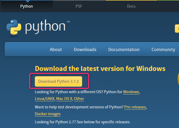
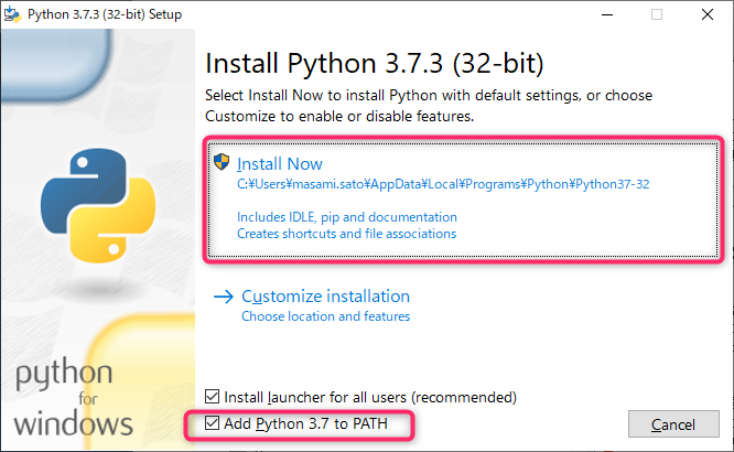
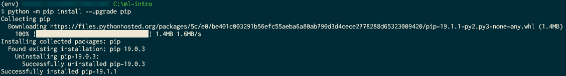
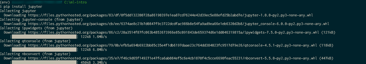
- 投稿日:2019-07-07T15:18:15+09:00
Python+OCR(tesseract)の新しい学習データ(言語データ)を追加してみた
背景
Anaconda + python + tesseract でOCR環境を構築したのですが、
対応していない言語をOCRする必要が出てきました。
ということで、新たな言語の学習データを追加してみました。環境
MacOS Mojave ver10.14.4
Anaconda Navigator 1.9.7
※Anacondaのインストールは、こちらを参考にいたしました
JupiterNotebook 5.4.0実践
tesseract用の学習データ(「xxxx.traindeddata」)を入手して、指定のフォルダに格納します。
学習データの入手
https://github.com/tesseract-ocr/tesseract
7セグメント用(温度計等のデジタル数字)
https://github.com/arturaugusto/display_ocr
「letsgoditital」→「letsgodigital.traineddata」を入手学習データの格納場所
ダウンロードしてきた学習データを下記のフォルダに格納します。今回は、「letsgoditital」を格納しました。
/Users/xxx/anaconda3/share/tessdata/もし、格納場所がわからない場合は、下記のコードを一度実行してみましょう。
実行結果の一番下に
「TesseractError: (1, b'Error opening data file 〜〜」
という部分があるかと思います。これは、指定した学習データがないよというエラーです。
なので、こちらに学習データを格納してあげましょう。txt = tool.image_to_string( Image.open('./imagesFolder/num/567.png'), lang="letsgodigital", builder=pyocr.builders.TextBuilder(tesseract_layout=6) ) print( txt )実行結果TesseractError Traceback (most recent call last) <ipython-input-7-294dc4179e9d> in <module>() 2 Image.open('./imagesFolder/num/567.png'), 3 lang="letsgodigital", ----> 4 builder=pyocr.builders.TextBuilder(tesseract_layout=6) 5 ) 6 print( txt ) ~/anaconda3/lib/python3.6/site-packages/pyocr/tesseract.py in image_to_string(image, lang, builder) 378 configs=builder.tesseract_configs) 379 if status: --> 380 raise TesseractError(status, errors) 381 382 tested_files = [] TesseractError: (1, b'Error opening data file /Users/xxxx/anaconda3/share/tessdata/letsgodigital.traineddata\n Please make sure the TESSDATA_PREFIX environment variable is set to your "tessdata" directory.\nFailed loading language \'letsgodigital\'\nTesseract couldn\'t load any languages!\nCould not initialize tesseract.\n')学習データの確認
下記コードを使って、学習データが使えるようになっているか確認します!
from PIL import Image
import sys
import pyocr
import pyocr.builders

tools = pyocr.get_available_tools()
if len(tools) == 0:
    print("No OCR tool found")
    sys.exit(1)
# The tools are returned in the recommended order of usage
tool = tools[0]
print("Will use tool '%s'" % (tool.get_name()))
# Ex: Will use tool 'libtesseract'

langs = tool.get_available_languages()
print("Available languages: %s" % ", ".join(langs))
lang = langs[0]
print("Will use lang '%s'" % (lang))
結果はこちら。
無事7セグメント用デジタル数字(「letsgodigital」)が使用可能なのが確認できます。実行結果Will use tool 'Tesseract (sh)' Available languages: eng, jpn, letsgodigital, Will use lang 'afr'終わりに
以上、tesseractの初期セットにない学習データを追加してみました!これで、いろんな言語のOCRが可能になります!
- 投稿日:2019-07-07T15:18:15+09:00
Python+OCR(tesseract)で新しい学習データ(言語データ)を追加してみた
背景
Anaconda + python + tesseract でOCR環境を構築したのですが、
対応していない言語をOCRする必要が出てきました。
ということで、新たな言語の学習データを追加してみました。環境
MacOS Mojave ver10.14.4
Anaconda Navigator 1.9.7
※Anacondaのインストールは、こちらを参考にいたしました
JupiterNotebook 5.4.0実践
tesseract用の学習データ(「xxxx.traindeddata」)を入手して、指定のフォルダに格納します。
学習データの入手
各種言語データ
https://github.com/tesseract-ocr/tessdata
使用したい言語データ(xxx.traineddata)を入手します。7セグメント用(温度計等のデジタル数字)
https://github.com/arturaugusto/display_ocr
「letsgoditital」→「letsgodigital.traineddata」を入手学習データの格納場所
ダウンロードしてきた学習データを下記のフォルダに格納します。今回は、「letsgoditital」を格納しました。
/Users/xxx/anaconda3/share/tessdata/もし、格納場所がわからない場合は、下記のコードを一度実行してみましょう。
実行結果の一番下に
「TesseractError: (1, b'Error opening data file 〜〜」
という部分があるかと思います。これは、指定した学習データがないよというエラーです。
なので、こちらに学習データを格納してあげましょう。txt = tool.image_to_string( Image.open('./imagesFolder/num/567.png'), lang="letsgodigital", builder=pyocr.builders.TextBuilder(tesseract_layout=6) ) print( txt )実行結果TesseractError Traceback (most recent call last) <ipython-input-7-294dc4179e9d> in <module>() 2 Image.open('./imagesFolder/num/567.png'), 3 lang="letsgodigital", ----> 4 builder=pyocr.builders.TextBuilder(tesseract_layout=6) 5 ) 6 print( txt ) ~/anaconda3/lib/python3.6/site-packages/pyocr/tesseract.py in image_to_string(image, lang, builder) 378 configs=builder.tesseract_configs) 379 if status: --> 380 raise TesseractError(status, errors) 381 382 tested_files = [] TesseractError: (1, b'Error opening data file /Users/xxxx/anaconda3/share/tessdata/letsgodigital.traineddata\n Please make sure the TESSDATA_PREFIX environment variable is set to your "tessdata" directory.\nFailed loading language \'letsgodigital\'\nTesseract couldn\'t load any languages!\nCould not initialize tesseract.\n')学習データの確認
下記コードを使って、学習データが使えるようになっているか確認します!
from PIL import Image
import sys
import pyocr
import pyocr.builders

tools = pyocr.get_available_tools()
if len(tools) == 0:
    print("No OCR tool found")
    sys.exit(1)
# The tools are returned in the recommended order of usage
tool = tools[0]
print("Will use tool '%s'" % (tool.get_name()))
# Ex: Will use tool 'libtesseract'

langs = tool.get_available_languages()
print("Available languages: %s" % ", ".join(langs))
lang = langs[0]
print("Will use lang '%s'" % (lang))
結果はこちら。
無事7セグメント用デジタル数字(「letsgodigital」)が使用可能なのが確認できます。実行結果Will use tool 'Tesseract (sh)' Available languages: eng, jpn, letsgodigital, Will use lang 'afr'終わりに
以上、tesseractの初期セットにない学習データを追加してみました!これで、いろんな言語のOCRが可能になります!
- 投稿日:2019-07-07T14:56:01+09:00
Google Home miniにNature Remo miniから取得した室温を教えてもらう
はじめに
Google Home miniを購入したので、前から持っていたNature Remo miniと連携して、部屋の温度を教えてくれる機能を実装した。このような記事はすでにいくつかネット上に存在するが、次の点が気になったので改めて書くことにした。
- 情報が古くなって後述するDialogflowの使い方が変っている
- ローカルネットワーク内にサーバーを構築する必要がある
- Google HomeもNature Remoもインターネットからアクセス可能なAPIがあるため、実はローカルサーバーは不要である
- DockerでHerokuにデプロイできる仕組みがない
このためこの記事ではこれらが解決されて次のようになることを目指した。
- 執筆時点でのUIをキャプチャした(Dialogflowは所見ではごちゃごちゃしているので、解説とUIが違うと手間がかかる)
- サーバーアプリケーションはDockerで起動できるようにし、Herokuにデプロイすることで動作する
- サーバーアプリケーションはPython + Flaskで実装した
この記事で作ったプログラムは下記に置かれている。
この記事を読んで何か分かりにくいことや改善点を見つけた場合、気軽にコメントなどで教えてほしい。
準備
Nature Remoのアクセストークンの取得
https://home.nature.global/home へアクセスして
Generate access tokenを押せば発行される。
Herokuのアプリケーションを作成
https://dashboard.heroku.com/apps へアクセスして
New > Create new appを押せばよい。
そして
App nameはgoogle-home-nature-remoとしたが、この命名はすでに筆者が利用してしまったので別の名称にしなければならない。このApp nameは後にコマンドライン上やURL上で利用するので、別の名前にした場合はこの記事のいろいろな部分を適宜修正する必要がある。この命名がコマンドラインやURLで必要になった場合は、《App name》と表記する。
最後に
Create appを押す。これでアプリケーションがデプロイできるようになる。そしてアプリケーションのために環境変数を設定する。https://dashboard.heroku.com/apps/《App name》/settingsへアクセスし次のように環境変数を入れる。
NATURE_REMO_TOKENは先ほど発行したNature RemoのアクセストークンでありBASIC_AUTH_USERNAMEとBASIC_AUTH_PASSWORDはそれぞれGoogle Home(正確にはDialogflow)がこのHerokuアプリケーションにアクセスするためのBasic認証の情報である。これはURLが特定されると部屋の温度を取得される恐れがあるため、このように認証をかけておくことにする。サーバーアプリケーションのデプロイ
HerokuのDockerアプリケーションをデプロイする。次のような流れを行う。
git clone https://github.com/y-yu/google-home-nature-remo-temperature.gitcd google-home-nature-remo-temperatureheroku login
- もしCLIの
herokuがない場合はHomebrewなどで適宜インストールするheroku container:loginheroku container:push web -a 《App name》heroku container:release web -a 《App name》これでサーバーサイド側は完成のはずである。次のコマンドでテストするとよい。
$ curl -XPOST --basic -u "user:*******" https://google-home-nature-remo.herokuapp.com/temperature | jq
{
  "payload": {
    "google": {
      "expectUserResponse": false,
      "richResponse": {
        "items": [
          {
            "simpleResponse": {
              "textToSpeech": "現在の室温は24.39度です"
            }
          }
        ]
      }
    }
  }
}
このようなJSONが表示されれば成功である。
Google Assistantアプリケーションの作成
https://console.actions.google.com/ へアクセスし
New projectを押すと、次のような画面があらわれる。
言語を日本語、地域を日本にして
Create projectする。するとWelcomeページが表示される。
ここからGoogle Homeで呼びだすための設定をしていくので、上のタブの
Developを押す。Invocationの設定
左のタブに
Invocationというのがあるので、まずはこれを設定する。これは「OK, Google.○○○○○につないで」の○○○○○を決めることで、さきほど作ったアプリケーションを呼び出すことができるようになる。ここでは部屋の温度にした。
これで「OK, Google. 部屋の温度につないで」と言うとこのGoogle Assistantアプリケーションが起動するようになる。
Actionの追加
それではDialogflowを使ってどのようなときにどうするのかを定義していく。あらかじめゴールを述べておくと「このアプリケーションが起動した時に、さきほど作ったHerokuアプリケーションに問い合わせてその情報を発言する」というものである。
まずは左側のタブからActionを選び、Add actionを押す。
今回はbuilt-inではないので、Custom intentを作るため、画像のような
BUILDボタンを押してDialogflowへ移動する。Dialogflowの設定
次からは
Create new agentで新しい設定を作成し、適当な名前をつける。ここからDialogflowを設定していく。Default Welcome Intentの無効化
このアプリケーションはデフォルトで「OK, Google.
○○○○○につないで」の後にやることであるWelcome Intentが決っているが、今回このGoogle Assistantアプリケーションは温度を返す機能しかないため、このデフォルト機能は必要ない。
そこで上の画像のように
Eventsに設定してあったWelcomeを削除して空にしておく。Fulfillmentの設定
次にHerokuアプリケーションへ問い合わせる部分を定義する。左側のタブから
Fulfillmentを選び、WebhookをENABLEにする。そしてHeroku側の環境変数に従ってBasic認証の情報とアプリケーションのURLを入力する。
そして画面右下の
SAVEを押す。Intentの設定
Dialogflowの左側のタプから
Intentを押し、右上にあるCREATE INTENTを押す。Intent nameは適当に入れておけばよい。ここはユーザーのどういうアクションに対して何をするかを定義する部分であり、今回は機能が1つ(部屋の温度を返すだけ)なので、起動した瞬間にHerokuアプリケーションへ問い合わせてもらえばよい。
したがって、まずはEventを設定する。
このように
Welcomeを設定した。そして一番下にあるEnable webhook call for this intentを有効にすればHerokuアプリケーションへの問い合わせが行われる。Integrationsの設定
最後に追加したIntentをGoogle Homeで使う設定を書いておく。もう
Default Welcome Intentはいらないので削除し、いま作ったroom temperatureを入れる。
また
Auto-preview changesを入れておけば修正したときに、明示的な操作なく変更が適用されて便利である。ここでTESTボタンを押してシミュレーターでテストしてみる。
このようになれば成功である。この時点でもう部屋のGoogle Homeから利用できる状態にあるので、たとえばこの例では「OK, Google. 部屋の温度につないで」と言えばきちんと応答される。
おわりに
Google Homeアプリケーションの開発は、とにかく覚えることが多くて大変であった。この資料が他の方々の開発に役立てばよいと思う。
参考文献


