- 投稿日:2020-03-27T23:05:16+09:00
Rasa NLU で自然言語理解のおためし
NLU (Natural Language Understanding=自然言語理解) をやってみたくて、
https://tech.mof-mof.co.jp/blog/rasa-nlu-japanese.html
を参考にしながら、dockerで環境を作って、実際に動くところまでやってみる。
Docker環境構築
ホストマシン上でrasa用のディレクトリを作る。
$ mkdir rasa
$ cd rasa
$ vi Dockerfile
Dockerfile に、まずは python が動くimageのみを記述してみる。
FROM python:3.7-slim-stretchdocker-composeで動かしたいので docker-compose.yml を作成
$ vi docker-compose.ymldocker-compose.ymlversion: '2' services: rasa: container_name: rasa build: context: . volumes: - .:/appbuildする
$ docker-compose build
Building rasa
Step 1/1 : FROM python:3.7-slim-stretch
 ---> c9ec5ac0f580
Successfully built c9ec5ac0f580
Successfully tagged rasa-test_rasa:latest

$
python動くか確認。
$ docker-compose run --rm rasa bash
Creating network "rasa-test_default" with the default driver
root@c02085da1f5f:/# python --version
Python 3.7.7
root@c02085da1f5f:/#
動いた。
Rasaをインストール
https://tech.mof-mof.co.jp/blog/rasa-nlu-tutorial.html
を参考にrasa環境を作っていく
root@c02085da1f5f:/# pip install rasa
...(なんかいろいろインストールされる)

Successfully built sanic-jwt absl-py mattermostwrapper colorclass webexteamssdk SQLAlchemy terminaltables future gast termcolor wrapt PyYAML docopt pyrsistent
Failed to build ujson
Installing collected packages: ujson, certifi, six, pycparser, cffi, cryptography, future, python-telegram-bot, tqdm, tabulate, python-crfsuite, sklearn-crfsuite, dnspython, pymongo, ruamel.yaml, numpy, h5py, keras-applications, opt-einsum, grpcio, protobuf, absl-py, google-pasta, gast, termcolor, scipy, wrapt, keras-preprocessing, werkzeug, cachetools, pyasn1, pyasn1-modules, rsa, google-auth, chardet, urllib3, idna, requests, markdown, oauthlib, requests-oauthlib, google-auth-oauthlib, tensorboard, tensorflow-estimator, astor, tensorflow, python-dateutil, PyYAML, docopt, pykwalify, zipp, importlib-metadata, pyrsistent, attrs, jsonschema, greenlet, gevent, redis, PyJWT, sanic-jwt, cloudpickle, kafka-python, rocketchat-API, joblib, scikit-learn, pysocks, pytz, twilio, cycler, pyparsing, kiwisolver, matplotlib, mattermostwrapper, multidict, psycopg2-binary, colorclass, aiofiles, rfc3986, hstspreload, hpack, hyperframe, h2, h11, sniffio, httpx, httptools, uvloop, websockets, sanic, requests-toolbelt, webexteamssdk, httplib2, oauth2client, python-engineio, tzlocal, apscheduler, async-generator, wcwidth, prompt-toolkit, questionary, fbmessenger, sanic-plugins-framework, sanic-cors, humanfriendly, coloredlogs, colorhash, jsonpickle, SQLAlchemy, async-timeout, yarl, aiohttp, pydot, packaging, rasa-sdk, python-socketio, tensorflow-hub, decorator, tensorflow-probability, typeguard, tensorflow-addons, terminaltables, networkx, jmespath, docutils, botocore, s3transfer, boto3, slackclient, pika, rasa
    Running setup.py install for ujson ... error
    ERROR: Command errored out with exit status 1:
     command: /usr/local/bin/python -u -c 'import sys, setuptools, tokenize; sys.argv[0] = '"'"'/tmp/pip-install-ingvl92n/ujson/setup.py'"'"'; __file__='"'"'/tmp/pip-install-ingvl92n/ujson/setup.py'"'"';f=getattr(tokenize, '"'"'open'"'"', open)(__file__);code=f.read().replace('"'"'\r\n'"'"', '"'"'\n'"'"');f.close();exec(compile(code, __file__, '"'"'exec'"'"'))' install --record /tmp/pip-record-46isinhm/install-record.txt --single-version-externally-managed --compile --install-headers /usr/local/include/python3.7m/ujson
         cwd: /tmp/pip-install-ingvl92n/ujson/
    Complete output (12 lines):
    Warning: 'classifiers' should be a list, got type 'filter'
    running install
    running build
    running build_ext
    building 'ujson' extension
    creating build
    creating build/temp.linux-x86_64-3.7
    creating build/temp.linux-x86_64-3.7/python
    creating build/temp.linux-x86_64-3.7/lib
    gcc -pthread -Wno-unused-result -Wsign-compare -DNDEBUG -g -fwrapv -O3 -Wall -fPIC -I./python -I./lib -I/usr/local/include/python3.7m -c ./python/ujson.c -o build/temp.linux-x86_64-3.7/./python/ujson.o -D_GNU_SOURCE
    unable to execute 'gcc': No such file or directory
    error: command 'gcc' failed with exit status 1
    ----------------------------------------
ERROR: Command errored out with exit status 1: /usr/local/bin/python -u -c 'import sys, setuptools, tokenize; sys.argv[0] = '"'"'/tmp/pip-install-ingvl92n/ujson/setup.py'"'"'; __file__='"'"'/tmp/pip-install-ingvl92n/ujson/setup.py'"'"';f=getattr(tokenize, '"'"'open'"'"', open)(__file__);code=f.read().replace('"'"'\r\n'"'"', '"'"'\n'"'"');f.close();exec(compile(code, __file__, '"'"'exec'"'"'))' install --record /tmp/pip-record-46isinhm/install-record.txt --single-version-externally-managed --compile --install-headers /usr/local/include/python3.7m/ujson Check the logs for full command output.
root@c02085da1f5f:/#
なんかエラー出た。
unable to execute 'gcc': No such file or directoryってことなので、それっぽいのをインストールするroot@c02085da1f5f:/# apt-get update -q -y && apt-get install -q -y build-essential ...(なんかいろいろインストールされる) update-alternatives: using /usr/bin/g++ to provide /usr/bin/c++ (c++) in auto mode Setting up build-essential (12.3) ... Processing triggers for libc-bin (2.24-11+deb9u4) ... root@c02085da1f5f:/#もっかいrasaのインストールにチャレンジ
root@c02085da1f5f:/# pip install rasa
...(なんかいろいろインストールされる)

Successfully built ujson
Installing collected packages: six, absl-py, cycler, python-dateutil, kiwisolver, numpy, pyparsing, matplotlib, docopt, PyYAML, pykwalify, protobuf, tensorflow-hub, kafka-python, pytz, multidict, pysocks, urllib3, certifi, idna, chardet, requests, PyJWT, twilio, fbmessenger, ruamel.yaml, yarl, attrs, async-timeout, aiohttp, slackclient, terminaltables, aiofiles, httptools, websockets, ujson, h11, hpack, hyperframe, h2, sniffio, rfc3986, hstspreload, httpx, uvloop, sanic, sanic-plugins-framework, sanic-cors, humanfriendly, coloredlogs, rasa-sdk, tzlocal, apscheduler, packaging, typeguard, tensorflow-addons, greenlet, gevent, pika, scipy, google-pasta, astor, termcolor, wrapt, grpcio, pyasn1, pyasn1-modules, rsa, cachetools, google-auth, werkzeug, markdown, oauthlib, requests-oauthlib, google-auth-oauthlib, tensorboard, h5py, keras-applications, tensorflow-estimator, keras-preprocessing, opt-einsum, gast, tensorflow, cloudpickle, decorator, tensorflow-probability, dnspython, pymongo, python-engineio, joblib, scikit-learn, httplib2, oauth2client, SQLAlchemy, requests-toolbelt, future, webexteamssdk, sanic-jwt, wcwidth, prompt-toolkit, colorhash, colorclass, tqdm, rocketchat-API, jmespath, docutils, botocore, s3transfer, boto3, questionary, zipp, importlib-metadata, pyrsistent, jsonschema, mattermostwrapper, jsonpickle, python-socketio, redis, pydot, networkx, pycparser, cffi, cryptography, python-telegram-bot, psycopg2-binary, async-generator, python-crfsuite, tabulate, sklearn-crfsuite, rasa
Successfully installed PyJWT-1.7.1 PyYAML-5.3.1 SQLAlchemy-1.3.15 absl-py-0.9.0 aiofiles-0.4.0 aiohttp-3.6.2 apscheduler-3.6.3 astor-0.8.1 async-generator-1.10 async-timeout-3.0.1 attrs-19.3.0 boto3-1.12.30 botocore-1.15.30 cachetools-4.0.0 certifi-2019.11.28 cffi-1.14.0 chardet-3.0.4 cloudpickle-1.2.2 colorclass-2.2.0 coloredlogs-10.0 colorhash-1.0.2 cryptography-2.8 cycler-0.10.0 decorator-4.4.2 dnspython-1.16.0 docopt-0.6.2 docutils-0.15.2 fbmessenger-6.0.0 future-0.18.2 gast-0.2.2 gevent-1.4.0 google-auth-1.12.0 google-auth-oauthlib-0.4.1 google-pasta-0.2.0 greenlet-0.4.15 grpcio-1.27.2 h11-0.8.1 h2-3.2.0 h5py-2.10.0 hpack-3.0.0 hstspreload-2020.3.25 httplib2-0.17.0 httptools-0.1.1 httpx-0.9.3 humanfriendly-8.1 hyperframe-5.2.0 idna-2.9 importlib-metadata-1.5.2 jmespath-0.9.5 joblib-0.14.1 jsonpickle-1.3 jsonschema-3.2.0 kafka-python-1.4.7 keras-applications-1.0.8 keras-preprocessing-1.1.0 kiwisolver-1.1.0 markdown-3.2.1 matplotlib-3.1.3 mattermostwrapper-2.2 multidict-4.7.5 networkx-2.4 numpy-1.18.2 oauth2client-4.1.3 oauthlib-3.1.0 opt-einsum-3.2.0 packaging-19.0 pika-1.1.0 prompt-toolkit-2.0.10 protobuf-3.11.3 psycopg2-binary-2.8.4 pyasn1-0.4.8 pyasn1-modules-0.2.8 pycparser-2.20 pydot-1.4.1 pykwalify-1.7.0 pymongo-3.8.0 pyparsing-2.4.6 pyrsistent-0.16.0 pysocks-1.7.1 python-crfsuite-0.9.7 python-dateutil-2.8.1 python-engineio-3.11.2 python-socketio-4.4.0 python-telegram-bot-11.1.0 pytz-2019.3 questionary-1.5.1 rasa-1.9.2 rasa-sdk-1.9.0 redis-3.4.1 requests-2.23.0 requests-oauthlib-1.3.0 requests-toolbelt-0.9.1 rfc3986-1.3.2 rocketchat-API-0.6.36 rsa-4.0 ruamel.yaml-0.15.100 s3transfer-0.3.3 sanic-19.12.2 sanic-cors-0.10.0.post3 sanic-jwt-1.3.2 sanic-plugins-framework-0.9.2 scikit-learn-0.22.2.post1 scipy-1.4.1 six-1.14.0 sklearn-crfsuite-0.3.6 slackclient-2.5.0 sniffio-1.1.0 tabulate-0.8.7 tensorboard-2.1.1 tensorflow-2.1.0 tensorflow-addons-0.8.3 tensorflow-estimator-2.1.0 tensorflow-hub-0.7.0 tensorflow-probability-0.7.0 termcolor-1.1.0 terminaltables-3.1.0 tqdm-4.31.1 twilio-6.26.3 typeguard-2.7.1 tzlocal-2.0.0 ujson-1.35 urllib3-1.25.8 uvloop-0.14.0 wcwidth-0.1.9 webexteamssdk-1.1.1 websockets-8.1 werkzeug-1.0.0 wrapt-1.12.1 yarl-1.4.2 zipp-3.1.0
root@c02085da1f5f:/#
インストールできた。
次はrasaのinit。
の前に、作業ディレクトリを移動する。/ 直下でなんかファイルができると気持ち悪いので。
root@c02085da1f5f:/# pwd
/
root@c02085da1f5f:/# ls -al
total 88
drwxr-xr-x   1 root root 4096 Mar 27 08:25 .
drwxr-xr-x   1 root root 4096 Mar 27 08:25 ..
-rwxr-xr-x   1 root root    0 Mar 27 08:25 .dockerenv
drwxr-xr-x   4 root root  128 Mar 27 08:22 app
drwxr-xr-x   1 root root 4096 Mar 27 08:33 bin
drwxr-xr-x   2 root root 4096 Feb  1 17:09 boot
drwxr-xr-x   5 root root  360 Mar 27 08:25 dev
drwxr-xr-x   1 root root 4096 Mar 27 08:33 etc
drwxr-xr-x   2 root root 4096 Feb  1 17:09 home
drwxr-xr-x   1 root root 4096 Mar 27 08:33 lib
drwxr-xr-x   2 root root 4096 Feb 24 00:00 lib64
drwxr-xr-x   2 root root 4096 Feb 24 00:00 media
drwxr-xr-x   2 root root 4096 Feb 24 00:00 mnt
drwxr-xr-x   2 root root 4096 Feb 24 00:00 opt
dr-xr-xr-x 228 root root    0 Mar 27 08:25 proc
drwx------   1 root root 4096 Mar 27 08:27 root
drwxr-xr-x   3 root root 4096 Feb 24 00:00 run
drwxr-xr-x   2 root root 4096 Feb 24 00:00 sbin
drwxr-xr-x   2 root root 4096 Feb 24 00:00 srv
dr-xr-xr-x  13 root root    0 Mar 27 08:25 sys
drwxrwxrwt   1 root root 4096 Mar 27 08:36 tmp
drwxr-xr-x   1 root root 4096 Feb 24 00:00 usr
drwxr-xr-x   1 root root 4096 Feb 24 00:00 var
root@c02085da1f5f:/# cd app/
root@c02085da1f5f:/app# ls -al
total 12
drwxr-xr-x 4 root root  128 Mar 27 08:22 .
drwxr-xr-x 1 root root 4096 Mar 27 08:25 ..
-rw-r--r-- 1 root root   29 Mar 27 08:20 Dockerfile
-rw-r--r-- 1 root root  112 Mar 27 08:22 docker-compose.yml
root@c02085da1f5f:/app#
/app で作業する。
rasa init する
root@c02085da1f5f:/app# rasa init --no-prompt
Welcome to Rasa! ?

To get started quickly, an initial project will be created.
If you need some help, check out the documentation at https://rasa.com/docs/rasa.

Created project directory at '/app'.
Finished creating project structure.
Training an initial model...
Training Core model...

(なんやかんや)

2020-03-27 08:46:25 INFO     rasa.nlu.model  - Successfully saved model into '/tmp/tmp4p2k58s6/nlu'
NLU model training completed.
Your Rasa model is trained and saved at '/app/models/20200327-084527.tar.gz'.
If you want to speak to the assistant, run 'rasa shell' at any time inside the project directory.
root@c02085da1f5f:/app#
init できたっぽい。
ディレクトリ内を見てみる。
root@c02085da1f5f:/app# ls -al
total 32
drwxr-xr-x 14 root root  448 Mar 27 08:46 .
drwxr-xr-x  1 root root 4096 Mar 27 08:25 ..
-rw-r--r--  1 root root   29 Mar 27 08:20 Dockerfile
-rw-r--r--  1 root root    0 Mar 27 08:36 __init__.py
drwxr-xr-x  4 root root  128 Mar 27 08:45 __pycache__
-rw-r--r--  1 root root  757 Mar 27 08:36 actions.py
-rw-r--r--  1 root root  622 Mar 27 08:36 config.yml
-rw-r--r--  1 root root  938 Mar 27 08:36 credentials.yml
drwxr-xr-x  4 root root  128 Mar 27 08:45 data
-rw-r--r--  1 root root  112 Mar 27 08:22 docker-compose.yml
-rw-r--r--  1 root root  549 Mar 27 08:36 domain.yml
-rw-r--r--  1 root root 1456 Mar 27 08:36 endpoints.yml
drwxr-xr-x  3 root root   96 Mar 27 08:46 models
drwxr-xr-x  3 root root   96 Mar 27 08:45 tests
root@c02085da1f5f:/app#
なんか色々増えてる。
参考にした記事と同様に、まずは会話してみる。
root@c02085da1f5f:/app# rasa shell
2020-03-27 08:54:07 INFO     root  - Connecting to channel 'cmdline' which was specified by the '--connector' argument. Any other channels will be ignored. To connect to all given channels, omit the '--connector' argument.
2020-03-27 08:54:07 INFO     root  - Starting Rasa server on http://localhost:5005
2020-03-27 08:54:08.593814: E tensorflow/stream_executor/cuda/cuda_driver.cc:351] failed call to cuInit: UNKNOWN ERROR (303)
Bot loaded. Type a message and press enter (use '/stop' to exit):
Your input ->  hello
Hey! How are you?
Your input ->  /stop
2020-03-27 08:54:31 INFO     root  - Killing Sanic server now.
root@c02085da1f5f:/app#
おお。できてる。
日本語に対応する
https://tech.mof-mof.co.jp/blog/rasa-nlu-japanese.html
次にこの記事に戻って日本語対応してみる。
まずは
data/nlu.mdの一番下にデータを追加してみる。$ vi data/nlu.mddata/nlu.md## intent:restaurant_ja - 渋谷で美味しいイタリアンない? - 和食食べたいんだけど、六本木におすすめある? - 今度麻布行くんだけど、フレンチのお店教えて上記記事だとmecabをやめてspaCyを使っているようなので、mecabを飛ばしてspaCyでやってみる。
config.yml にデフォルト設定があるようなので、一旦全部消して以下を書いてみる。
config.ymlpipeline: # - name: “tokenizer_whitespace” - name: “nlp_spacy” - name: “tokenizer_spacy” - name: “CRFEntityExtractor” - name: “ner_crf” - name: “ner_synonyms” - name: “intent_featurizer_count_vectors” - name: “intent_classifier_tensorflow_embedding”学習させてみる。
root@c02085da1f5f:/app# rasa train nlu
The config file 'config.yml' is missing mandatory parameters: 'language'. Add missing parameters to config file and try again.
root@c02085da1f5f:/app#
config.yml に languageが無いよって。
上記記事だとja_ginzaにしているようなので、端折って config.yml の一番上に ja_ginza を追加してみる。
config.ymllanguage: ja_ginzaもういっかいコマンドを叩いてみる。
root@c02085da1f5f:/app# rasa train nlu
Training NLU model...
Traceback (most recent call last):
  File "/usr/local/lib/python3.7/site-packages/rasa/nlu/registry.py", line 173, in get_component_class
    return class_from_module_path(component_name)
  File "/usr/local/lib/python3.7/site-packages/rasa/utils/common.py", line 211, in class_from_module_path
    raise ImportError(f"Cannot retrieve class from path {module_path}.")
ImportError: Cannot retrieve class from path “nlp_spacy”.

(なんやかんや)
nlp_spacyが云々で怒られている。
spaCy入れてないもんね。
spaCy入れてみる。
root@c02085da1f5f:/app# pip install spacy

(なんやかんや)

Successfully installed blis-0.4.1 catalogue-1.0.0 cymem-2.0.3 murmurhash-1.0.2 plac-1.1.3 preshed-3.0.2 spacy-2.2.4 srsly-1.0.2 thinc-7.4.0 tqdm-4.43.0 wasabi-0.6.0
root@c02085da1f5f:/app#
入った。
GiNZAの日本語処理ライブラリ?があるようなので、インストールする。
root@c02085da1f5f:/app# pip install "https://github.com/megagonlabs/ginza/releases/download/latest/ginza-latest.tar.gz"
Collecting https://github.com/megagonlabs/ginza/releases/download/latest/ginza-latest.tar.gz

(なんやかんや)

Successfully built ginza ja-ginza SudachiDict-core
Installing collected packages: ja-ginza, sortedcontainers, Cython, dartsclone, SudachiPy, SudachiDict-core, ginza
Successfully installed Cython-0.29.16 SudachiDict-core-20190927 SudachiPy-0.4.3 dartsclone-0.9.0 ginza-2.2.1 ja-ginza-2.2.0 sortedcontainers-2.1.0
root@c02085da1f5f:/app#
インストールできた。
これで準備できたか?
もう一回コマンドを叩く。
root@c02085da1f5f:/app# rasa train nlu
Training NLU model...
Traceback (most recent call last):
  File "/usr/local/lib/python3.7/site-packages/rasa/nlu/registry.py", line 173, in get_component_class
    return class_from_module_path(component_name)
  File "/usr/local/lib/python3.7/site-packages/rasa/utils/common.py", line 211, in class_from_module_path
    raise ImportError(f"Cannot retrieve class from path {module_path}.")
ImportError: Cannot retrieve class from path “nlp_spacy”.

During handling of the above exception, another exception occurred:

Traceback (most recent call last):
  File "/usr/local/bin/rasa", line 8, in <module>
    sys.exit(main())
  File "/usr/local/lib/python3.7/site-packages/rasa/__main__.py", line 91, in main
    cmdline_arguments.func(cmdline_arguments)
  File "/usr/local/lib/python3.7/site-packages/rasa/cli/train.py", line 140, in train_nlu
    persist_nlu_training_data=args.persist_nlu_data,
  File "/usr/local/lib/python3.7/site-packages/rasa/train.py", line 414, in train_nlu
    persist_nlu_training_data,
  File "uvloop/loop.pyx", line 1456, in uvloop.loop.Loop.run_until_complete
  File "/usr/local/lib/python3.7/site-packages/rasa/train.py", line 445, in _train_nlu_async
    persist_nlu_training_data=persist_nlu_training_data,
  File "/usr/local/lib/python3.7/site-packages/rasa/train.py", line 474, in _train_nlu_with_validated_data
    persist_nlu_training_data=persist_nlu_training_data,
  File "/usr/local/lib/python3.7/site-packages/rasa/nlu/train.py", line 74, in train
    trainer = Trainer(nlu_config, component_builder)
  File "/usr/local/lib/python3.7/site-packages/rasa/nlu/model.py", line 142, in __init__
    components.validate_requirements(cfg.component_names)
  File "/usr/local/lib/python3.7/site-packages/rasa/nlu/components.py", line 51, in validate_requirements
    component_class = registry.get_component_class(component_name)
  File "/usr/local/lib/python3.7/site-packages/rasa/nlu/registry.py", line 199, in get_component_class
    raise ModuleNotFoundError(exception_message)
ModuleNotFoundError: Cannot find class '“nlp_spacy”' from global namespace. Please check that there is no typo in the class name and that you have imported the class into the global namespace.
root@c02085da1f5f:/app#
なんか怒られた。
Cannot find class '“nlp_spacy”'ってなんだろ。
ModuleNotFoundError: Cannot find class '“nlp_spacy”' from global namespace. Please check that there is no typo in the class name and that you have imported the class into the global namespace.でググってみる。https://github.com/RasaHQ/rasa/blob/master/rasa/nlu/registry.py
このページが一番上に出てきた。
https://github.com/RasaHQ/rasa/blob/master/rasa/nlu/registry.py#L101
old_style_names?"nlp_spacy": "SpacyNLP",こんな感じの対応付けが定義されている。
さっきconfig.ymlに書いたのが、
nlp_spacyだからSpacyNLPに変更してみる。config.ymllanguage: ja_ginza pipeline: # - name: “tokenizer_whitespace” - name: "SpacyNLP" # ←ここを変更 - name: "tokenizer_spacy" - name: "CRFEntityExtractor" - name: "ner_crf" - name: "ner_synonyms" - name: "intent_featurizer_count_vectors" - name: "intent_classifier_tensorflow_embedding"再度コマンドを叩く。
root@c02085da1f5f:/app# rasa train nlu
Training NLU model...

(なんやかんや)

ModuleNotFoundError: Cannot find class '“SpacyNLP”' from global namespace. Please check that there is no typo in the class name and that you have imported the class into the global namespace.
“SpacyNLP”??あ、コピペしたらダブルクオートがおかしいのか。
ダブルクオートを治す。
config.ymllanguage: ja_ginza pipeline: # - name: “tokenizer_whitespace” - name: "nlp_spacy" - name: "tokenizer_spacy" - name: "CRFEntityExtractor" - name: "ner_crf" - name: "ner_synonyms" - name: "intent_featurizer_count_vectors" - name: "intent_classifier_tensorflow_embedding"もういっかいコマンド叩く。
root@c02085da1f5f:/app# rasa train nlu
Training NLU model...

(なんやかんや)

oblib, which can be installed with: pip install joblib. If this warning is raised when loading pickled models, you may need to re-serialize those models with scikit-learn 0.21+.
  warnings.warn(msg, category=FutureWarning)
2020-03-27 09:15:20 INFO     rasa.nlu.model  - Successfully saved model into '/tmp/tmpn4xtb3h7/nlu'
NLU model training completed.
Your Rasa model is trained and saved at '/app/models/nlu-20200327-091520.tar.gz'.
root@c02085da1f5f:/app#
お、やっと動いた。
rasa shell nluで intent が取れれば成功?root@c02085da1f5f:/app# rasa shell nlu 2020-03-27 09:16:26 INFO rasa.nlu.components - Added 'SpacyNLP' to component cache. Key 'SpacyNLP-ja_ginza'. /usr/local/lib/python3.7/site-packages/sklearn/externals/joblib/__init__.py:15: FutureWarning: sklearn.externals.joblib is deprecated in 0.21 and will be removed in 0.23. Please import this functionality directly from joblib, which can be installed with: pip install joblib. If this warning is raised when loading pickled models, you may need to re-serialize those models with scikit-learn 0.21+. warnings.warn(msg, category=FutureWarning) 2020-03-27 09:16:26.359929: E tensorflow/stream_executor/cuda/cuda_driver.cc:351] failed call to cuInit: UNKNOWN ERROR (303) /usr/local/lib/python3.7/site-packages/rasa/nlu/classifiers/diet_classifier.py:864: FutureWarning: 'EmbeddingIntentClassifier' is deprecated and will be removed in version 2.0. Use 'DIETClassifier' instead. model=model, NLU model loaded. Type a message and press enter to parse it. Next message: 六本木のイタリアン教えて { "intent": { "name": "restaurant_ja", "confidence": 0.48260971903800964 }, "entities": [], "intent_ranking": [ { "name": "restaurant_ja", "confidence": 0.48260971903800964 }, { "name": "affirm", "confidence": 0.1126396581530571 }, { "name": "greet", "confidence": 0.09804855287075043 }, { "name": "goodbye", "confidence": 0.08541827648878098 }, { "name": "mood_great", "confidence": 0.07586738467216492 }, { "name": "deny", "confidence": 0.06578702479600906 }, { "name": "bot_challenge", "confidence": 0.05436018109321594 }, { "name": "mood_unhappy", "confidence": 0.025269268080592155 } ], "text": "六本木のイタリアン教えて" } Next message:お、それっぽい。intentのスコア低いけど、こんなもん?
固有表現もやってみよう。
data/nlu.mdの日本語の箇所を下記のように書き換えて、data/nlu.md## intent:restaurant_ja - [渋谷](location)で美味しい[イタリアン](restaurant_type)ない? - [和食](restaurant_type)食べたいんだけど、[六本木](location)におすすめある? - 今度[麻布](location)行くんだけど、[フレンチ](restaurant_type)のお店教えて学習させて、
root@c02085da1f5f:/app# rasa train nlu
Training NLU model...

(なんやかんや)

2020-03-27 13:46:37 INFO     rasa.nlu.model  - Finished training component.
/usr/local/lib/python3.7/site-packages/sklearn/externals/joblib/__init__.py:15: FutureWarning: sklearn.externals.joblib is deprecated in 0.21 and will be removed in 0.23. Please import this functionality directly from joblib, which can be installed with: pip install joblib. If this warning is raised when loading pickled models, you may need to re-serialize those models with scikit-learn 0.21+.
  warnings.warn(msg, category=FutureWarning)
2020-03-27 13:46:37 INFO     rasa.nlu.model  - Successfully saved model into '/tmp/tmpy7tqyrsb/nlu'
NLU model training completed.
Your Rasa model is trained and saved at '/app/models/nlu-20200327-134637.tar.gz'.
root@c02085da1f5f:/app#
shell を叩いてみる。
root@c02085da1f5f:/app# rasa shell nlu
2020-03-27 13:47:07 INFO     rasa.nlu.components  - Added 'SpacyNLP' to component cache. Key 'SpacyNLP-ja_ginza'.
/usr/local/lib/python3.7/site-packages/sklearn/externals/joblib/__init__.py:15: FutureWarning: sklearn.externals.joblib is deprecated in 0.21 and will be removed in 0.23. Please import this functionality directly from joblib, which can be installed with: pip install joblib. If this warning is raised when loading pickled models, you may need to re-serialize those models with scikit-learn 0.21+.
  warnings.warn(msg, category=FutureWarning)
2020-03-27 13:47:07.924760: E tensorflow/stream_executor/cuda/cuda_driver.cc:351] failed call to cuInit: UNKNOWN ERROR (303)
/usr/local/lib/python3.7/site-packages/rasa/nlu/classifiers/diet_classifier.py:864: FutureWarning: 'EmbeddingIntentClassifier' is deprecated and will be removed in version 2.0. Use 'DIETClassifier' instead.
  model=model,
NLU model loaded. Type a message and press enter to parse it.
Next message:
渋谷で美味しいイタリアンない?
{
  "intent": {
    "name": "restaurant_ja",
    "confidence": 0.9823814034461975
  },
  "entities": [
    {
      "start": 0,
      "end": 2,
      "value": "渋谷",
      "entity": "location",
      "confidence": 0.7429793877231764,
      "extractor": "CRFEntityExtractor"
    },
    {
      "start": 7,
      "end": 12,
      "value": "イタリアン",
      "entity": "restaurant_type",
      "confidence": 0.7588623133724827,
      "extractor": "CRFEntityExtractor"
    },
    {
      "start": 0,
      "end": 2,
      "value": "渋谷",
      "entity": "location",
      "confidence": 0.7429793877231764,
      "extractor": "CRFEntityExtractor"
    },
    {
      "start": 7,
      "end": 12,
      "value": "イタリアン",
      "entity": "restaurant_type",
      "confidence": 0.7588623133724827,
      "extractor": "CRFEntityExtractor"
    }
  ],
  "intent_ranking": [
    {
      "name": "restaurant_ja",
      "confidence": 0.9823814034461975
    },
    {
      "name": "mood_great",
      "confidence": 0.008284788578748703
    },
    {
      "name": "deny",
      "confidence": 0.006644146051257849
    },
    {
      "name": "greet",
      "confidence": 0.001571052591316402
    },
    {
      "name": "bot_challenge",
      "confidence": 0.0006475948612205684
    },
    {
      "name": "affirm",
      "confidence": 0.00034828390926122665
    },
    {
      "name": "mood_unhappy",
      "confidence": 8.46567636472173e-05
    },
    {
      "name": "goodbye",
      "confidence": 3.805106462095864e-05
    }
  ],
  "text": "渋谷で美味しいイタリアンない?"
}
Next message:
おお。記事みたいな出力になった。
記事とは違って日本語は文字化けしてないけど。
環境ができて動くところまで見れたので、今回はここまで。
今後は教師データを増やす方法を考える。追記
ここまでの成果として、pip で install したライブラリを requirements.txt にして、build したら勝手にインストールされるように Dockerfile に処理を追記しておいた。
requirements.txtrasa==1.9.2 spacy==2.2.4FROM python:3.7-slim-stretch RUN apt-get update -q -y && \ apt-get install -q -y \ build-essential ADD ./requirements.txt requirements.txt RUN pip install -r requirements.txt RUN pip install "https://github.com/megagonlabs/ginza/releases/download/latest/ginza-latest.tar.gz" ADD . /app WORKDIR /appんで、build して
$ docker-compose build動かす
$ docker-compose run --rm rasa bash
root@56ff2c2f2f38:/app#
追記2
github で公開した
https://github.com/booink/rasa-trial
追記3
ginzaのインストールはpip経由で(3.0から)できるようになったようなので、requirements.txtにginzaを追記してDockerfileから該当箇所を削除した。
https://github.com/booink/rasa-trial/commit/eb8e020d70ad8d92e29c628008d550d214bcc14c
- 投稿日:2020-03-27T22:26:17+09:00
1次元移流方程式を有限要素法で解いてみる.py
1次元移流方程式をSUPG(Streamline Upwind/Petrov-Galerkin)法に基づく安定化有限要素法によって解いてみます.
言語はPythonを用います.使用したバージョンは Python 3.6.1です.参考文献:
計算力学(第2版)-有限要素法の基礎(森北出版)
第3版 有限要素法による流れのシミュレーション OpenMPに基づくFortranソースコード付(丸善出版)1次元移流方程式
1次元移流方程式は以下のような1階の偏微分方程式で表されます.
\cfrac{\partial f}{\partial t} + u\ \cfrac{\partial f}{\partial x} = 0ここで,$f$ は移流される物理量(例えば濃度),$u$ は移流速度です.
安定化有限要素法による離散化
解析領域 $\Omega$ を$M$ 個の1次要素の要素領域 $\Omega_e$に分割すると以下の離散化方程式が得られます.
\int_\Omega \omega\ \cfrac{\partial f}{\partial t}\ d\Omega\ + \int_\Omega \omega\ u\ \cfrac{\partial f}{\partial x}\ d\Omega\ + \sum_{e = 1}^M\int_{\Omega_e} \tau_e\ u\ \cfrac{\partial \omega}{\partial x}\left(\cfrac{\partial f}{\partial t}\ + u\ \cfrac{\partial f}{\partial x}\right)\ d\Omega = 0ここで,$\omega$ は重み関数,$\tau_e$ は安定化パラメータであり,一般的に非定常問題の場合は要素長 $h_e$ と時間刻み$\Delta t$ を用いて
\tau_e = \left(\left( \cfrac{2}{\Delta t}\right)^2 + \left(\cfrac{2|u|}{h_e}\right)^2\ \right)^{-\frac{1}{2}}と表されます.ある要素 $e$ に着目すると
\int_{\Omega_e} \omega\ \cfrac{\partial f}{\partial t}\ d\Omega\ + \int_{\Omega_e} \omega\ u\ \cfrac{\partial f}{\partial x}\ d\Omega\ + \int_{\Omega_e} \tau_e\ u\ \cfrac{\partial \omega}{\partial x}\left(\cfrac{\partial f}{\partial t}\ + u\ \cfrac{\partial f}{\partial x}\right)\ d\Omega = 0が得られます.2節点1次要素を用いて要素内の $\omega$, $f$ 及び $u$ をそれぞれ
\begin{align}
\omega(x) &= \cfrac{x_2^e - x}{h_e}\ \omega_1^e + \cfrac{x - x_1^e}{h_e}\ \omega_2^e\\
&=
\begin{pmatrix}
N_1^e & N_2^e
\end{pmatrix}
\begin{pmatrix}
\omega_1^e\\
\omega_2^e\\
\end{pmatrix}
= {\bf N}_e{\bf \omega}_e,
\end{align}
\begin{align} f(x) &= \cfrac{x_2^e - x}{h_e}\ f_1^e + \cfrac{x - x_1^e}{h_e}\ f_2^e\\ &= \begin{pmatrix} N_1^e & N_2^e \end{pmatrix} \begin{pmatrix} f_1^e\\ f_2^e\\ \end{pmatrix} = {\bf N}_e{\bf f}_e, \end{align}\begin{align} u(x) &= \cfrac{x_2^e - x}{h_e}\ u_1^e + \cfrac{x - x_1^e}{h_e}\ u_2^e\\ &= {\begin{pmatrix} N_1^e & N_2^e \end{pmatrix}} \begin{pmatrix} u_1^e\\ u_2^e\\ \end{pmatrix} = {\bf N}_e{\bf u}_e \end{align}と補間します.同様に $f$ の時間微分も
\begin{align}
\dot{f}(x) &= \cfrac{x_2^e - x}{h_e}\ \dot{f}_1^e + \cfrac{x - x_1^e}{h_e}\ \dot{f}_2^e\\
&=
{\begin{pmatrix}
N_1^e & N_2^e
\end{pmatrix}}
\begin{pmatrix}
\dot{f}_1^e\\
\dot{f}_2^e\\
\end{pmatrix}
= {\bf N}_e\dot{{\bf f}}_e
\end{align}
と補間します.これら代入すると以下の式が得られます.
\int_{\Omega_e} {\bf N}_e{\bf \omega}_e {\bf N}_e\dot{\bf f}_e\ d\Omega\
+ \int_{\Omega_e} {\bf N}_e{\bf \omega}_e\ {\bf N}_e{\bf u}_e\cfrac{\partial {\bf N}_e}{\partial x}\ {\bf f}_e\ d\Omega\
+ \int_{\Omega_e} \tau_e\ {\bf N}_e{\bf u}_e\cfrac{\partial {\bf N}_e}{\partial x}{\bf \omega}_e\left({\bf N}_e\dot{{\bf f}}_e\ + {\bf N}_e{\bf u}_e\cfrac{\partial {\bf N}_e}{\partial x}{\bf f}_e\right)\ d\Omega = 0
形状関数 $N$ の空間微分は
\begin{align}
\cfrac{\partial {\bf N}_e}{\partial x}
&=
{\begin{pmatrix}
\cfrac{\partial N_1^e}{\partial x} & \cfrac{\partial N_2^e}{\partial x}
\end{pmatrix}}
=
{\begin{pmatrix}
-\cfrac{1}{h_e} & \cfrac{1}{h_e}
\end{pmatrix}}
\end{align}
となり,要素内では一定値となります.
${\bf N}_ e\omega_e = ({\bf N}_ e \omega_e)^T = \omega_e^T{\bf N}_ e^T$ 等を用いて式変形していくと\omega_e^T\left(\int_{\Omega_e} {\bf N}_e^T{\bf N}_e\ d\Omega\ \dot{\bf f}_e\ + \int_{\Omega_e} {\bf N}_e^T\ {\bf N}_e{\bf u}_e\ \cfrac{\partial {\bf N}_e}{\partial x}\ d\Omega\ {\bf f}_e\ + \int_{\Omega_e} \tau_e\ \left(\cfrac{\partial {\bf N}_e}{\partial x}\right)^T{\bf u}_e^T{\bf N}_e^T{\bf N}_e\ d\Omega\ \dot{{\bf f}}_e\ + \int_{\Omega_e} \tau_e\ \left(\cfrac{\partial {\bf N}_e}{\partial x}\right)^T{\bf u}_e^T{\bf N}_e^T{\bf N}_e\ d\Omega\ {\bf u}_e\cfrac{\partial {\bf N}_e}{\partial x}\ {{\bf f}}_e\right)= 0となります.重み関数は任意に選んだ定数なので,有限要素方程式は以下のようになります.
\left({\bf M}_e + {\bf M}_{\delta e}\right)\ \dot{{\bf f}}_e + \left({\bf S}_e + {\bf S}_{\delta e}\right)\ {\bf f}_e = 0${\bf M}_ e$ は質量行列,${\bf S}_ e$ は移流行列,${\bf M}_ {\delta e}$, ${\bf S}_ {\delta e}$ はそれぞれSUPG項から生じる質量行列と移流行列です.
これらの行列は線座標を用いて求めることが可能であり,それぞれ{\bf M}_e = \int_{\Omega_e} {\bf N}_e^T{\bf N}_e\ d\Omega = \cfrac{h_e}{6} \begin{pmatrix} 2 & 1\\ 1 & 2 \end{pmatrix},\begin{align} {\bf A}_e &= \int_{\Omega_e} {\bf N}_e^T\ {\bf N}_e{\bf u}_e\cfrac{\partial {\bf N}_e}{\partial x}\ d\Omega\\ &= \int_{\Omega_e} {\bf N}_e^T\ {\bf N}_e\ d\Omega\ {\bf u}_e\cfrac{\partial {\bf N}_e}{\partial x}\\ &= \cfrac{h_e}{6} \begin{pmatrix} 2 & 1\\ 1 & 2 \end{pmatrix} \begin{pmatrix} u_1^e\\ u_2^e \end{pmatrix} \begin{pmatrix} -\cfrac{1}{h_e} & \cfrac{1}{h_e} \end{pmatrix}\\ &= \cfrac{1}{6} \begin{pmatrix} 2 & 1\\ 1 & 2 \end{pmatrix} \begin{pmatrix} -u_1^e & u_1^e\\ -u_2^e & u_2^e \end{pmatrix}\\ &= \cfrac{1}{6} \begin{pmatrix} -2u_1^e - u_2^e & 2u_1^e + u_2^e\\ -u_1^e - 2u_2^e & u_1^e + 2u_2^e \end{pmatrix}, \end{align}\begin{align} {\bf M}_{\delta e} &= \int_{\Omega_e} \tau_e\ \left(\cfrac{\partial {\bf N}_e}{\partial x}\right)^T{\bf u}_e^T{\bf N}_e^T{\bf N}_e\ d\Omega\\ &= \tau_e\ \left(\cfrac{\partial {\bf N}_e}{\partial x}\right)^T{\bf u}_e^T\ \int_{\Omega_e} {\bf N}_e^T{\bf N}_e\ d\Omega\\ &= \tau_e \begin{pmatrix} -\cfrac{1}{h_e}\\ \cfrac{1}{h_e} \end{pmatrix} \begin{pmatrix} u_1^e & u_2^e \end{pmatrix} \cfrac{h_e}{6} \begin{pmatrix} 2 & 1\\ 1 & 2 \end{pmatrix}\\ &= \cfrac{\tau_e}{6} \begin{pmatrix} -2u_1^e - u_2^e & -u_1^e - 2u_2^e\\ 2u_1^e + u_2^e & u_1^e + 2u_2^e \end{pmatrix}, \end{align}\begin{align} {\bf A}_{\delta e} &= \int_{\Omega_e} \tau_e\ \left(\cfrac{\partial {\bf N}_e}{\partial x}\right)^T{\bf u}_e^T{\bf N}_e^T{\bf N}_e\ d\Omega\ {\bf u}_e\cfrac{\partial {\bf N}_e}{\partial x}\\ &= \tau_e\ \left(\cfrac{\partial {\bf N}_e}{\partial x}\right)^T{\bf u}_e^T \int_{\Omega_e} {\bf N}_e^T{\bf N}_e\ d\Omega\ {\bf u}_e\cfrac{\partial {\bf N}_e}{\partial x}\\ &=\tau_e \begin{pmatrix} -\cfrac{1}{h_e}\\ \cfrac{1}{h_e} \end{pmatrix} \begin{pmatrix} u_1^e & u_2^e \end{pmatrix} \cfrac{h_e}{6} \begin{pmatrix} 2 & 1\\ 1 & 2 \end{pmatrix} \begin{pmatrix} u_1^e\\ u_2^e \end{pmatrix} \begin{pmatrix} -\cfrac{1}{h_e} & \cfrac{1}{h_e} \end{pmatrix}\\ &= \cfrac{\tau_e}{3h_e}\left({u_1^e}^2 + u_1^e u_2^e + {u_2^e}^2 \right) \begin{pmatrix} 1 & -1\\ -1 & 1 \end{pmatrix} \end{align}となります.これらを使って全体の有限要素方程式
\left({\bf M} + {\bf M}_{\delta}\right)\ \dot{{\bf f}} + \left({\bf S} + {\bf S}_{\delta}\right)\ {\bf f} = 0を組み立てていきます.時間方向の離散化にクランク・ニコルソン法を用いると
\left({\bf M} + {\bf M}_{\delta}\right)\ \cfrac{{\bf f}^{n+1} - {\bf f}^n}{\Delta t} + \left({\bf S} + {\bf S}_{\delta}\right)\ \cfrac{1}{2}\left({\bf f}^{n+1} + {\bf f}^n\right) = 0が得られます.$n$ は時間ステップです.さらに変形すると
\left(\cfrac{1}{\Delta t}\left({\bf M} + {\bf M}_{\delta}\right) + \cfrac{1}{2} \left({\bf S} + {\bf S}_{\delta}\right)\right) {\bf f}^{n+1}
=
\left(\cfrac{1}{\Delta t}\left({\bf M} + {\bf M}_{\delta}\right) - \cfrac{1}{2} \left({\bf S} + {\bf S}_{\delta}\right)\right) {\bf f}^n
となります.この式をよく見てみると,左辺が未知量,右辺は既知量で,${\bf A}{\bf x} = {\bf b}$ という連立1次方程式の形をしていることが分かります.つまり,この連立1次方程式を解けば次の時刻の物理量が得られるという事です.
Pythonによる実装
各要素ごとに質量・移流行列を求めて全体行列に足しこんでいきます.コードを以下に示します.なお,上記の式を愚直にコーディングしただけであり,連立1次方程式を解くためにNumPyのlinalg.solveを用いています.本来は高速化のために三重対角行列アルゴリズムや反復法などを用いるべきですが,今回は簡単のためlinalg.solveを用いています.
解析領域は$0 \le x \le 2$ とし,境界条件は $f(x = 0, t) = f(x = 2, t) = 0$ というディリクレ境界条件を与えます.
初期条件は$0 \le x \le 1$ で $f(x, t = 0) = \sin(\pi x)$,それ以外で $f(x, t = 0) = 0$ とします.移流速度は全領域で一様で $u = 1.0$ を与えます.実装やアニメーションの作成には以下のサイトを参考にしました.
【NumPy】連立方程式を解く numpy.linalg.solve
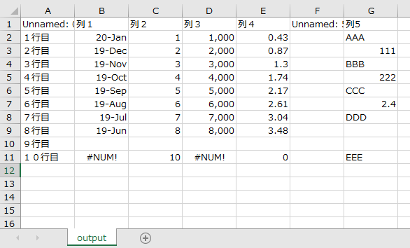
Pythonで波動方程式の数値計算 & 結果のアニメーション1d_advection.pyimport math import numpy as np import matplotlib.pyplot as plt import matplotlib.animation as animation # 各種定数の設定 dt = 0.005 # 時間刻み xmin = 0.0 xmax = 2.0 N = 200 dx = (xmax - xmin)/N # 空間刻み U = 1.0 # 移流速度 M = 200 # 変数の初期化 f = np.array([[0.0]*(N + 1) for i in range(M + 1)]) u = np.zeros([N + 1]) # マトリクスの初期化 A = np.array([[0.0]*(N + 1) for i in range(N + 1)]) b = np.array([0.0]*(N + 1)) # 初期条件 for i in range(N + 1): u[i] = U if i*dx <= 1.0: f[0, i] = math.sin(math.pi*i*dx) else: f[0, i] = 0.0 for ti in range(0, M): A.fill(0.0) b.fill(0.0) for i in range(N): u1 = u[i] u2 = u[i + 1] tau = 1.0/math.sqrt((2.0/dt)**2 + (2.0*U/dx)**2) # 質量行列 A[i ,i ] = A[i ,i ] + 1.0/dt*2.0/6.0*dx A[i ,i + 1] = A[i ,i + 1] + 1.0/dt*1.0/6.0*dx A[i + 1,i ] = A[i + 1,i ] + 1.0/dt*1.0/6.0*dx A[i + 1,i + 1] = A[i + 1,i + 1] + 1.0/dt*2.0/6.0*dx # 質量行列(SUPG) A[i ,i ] = A[i ,i ] + tau/dt/6.0*(-2.0*u1 - u2) A[i ,i + 1] = A[i ,i + 1] + tau/dt/6.0*(- u1 - 2.0*u2) A[i + 1,i ] = A[i + 1,i ] + tau/dt/6.0*( 2.0*u1 + u2) A[i + 1,i + 1] = A[i + 1,i + 1] + tau/dt/6.0*( u1 + 2.0*u2) # 移流行列 A[i ,i ] = A[i ,i ] + 0.5/6.0*(-2.0*u1 - u2) A[i ,i + 1] = A[i ,i + 1] + 0.5/6.0*( 2.0*u1 + u2) A[i + 1,i ] = A[i + 1,i ] + 0.5/6.0*(- u1 - 2.0*u2) A[i + 1,i + 1] = A[i + 1,i + 1] + 0.5/6.0*( u1 + 2.0*u2) # 移流行列(SUPG) A[i ,i ] = A[i ,i ] + 0.5*tau/3.0/dx*(u1**2 + u1*u2 + u2**2) A[i ,i + 1] = A[i ,i + 1] - 0.5*tau/3.0/dx*(u1**2 + u1*u2 + u2**2) A[i + 1,i ] = A[i + 1,i ] - 0.5*tau/3.0/dx*(u1**2 + u1*u2 + u2**2) A[i + 1,i + 1] = A[i + 1,i + 1] + 0.5*tau/3.0/dx*(u1**2 + u1*u2 + u2**2) for i in range(N): f1 = f[ti, i] f2 = f[ti, i + 1] u1 = u[i] u2 = u[i + 1] tau = 1.0/math.sqrt((2.0/dt)**2 + (2.0*U/dx)**2) # 質量行列 b[i ] = b[i ] + 1.0/dt*dx/6.0*(2.0*f1 + f2) b[i + 1] = b[i + 1] + 1.0/dt*dx/6.0*( f1 + 2.0*f2) # 質量行列(SUPG) b[i ] = b[i ] + tau/dt/6.0*((-2.0*u1 - u2)*f1 + (-u1 - 2.0*u2)*f2) b[i + 1] = b[i + 1] + tau/dt/6.0*(( 2.0*u1 + u2)*f1 + ( u1 + 2.0*u2)*f2) # 移流行列 b[i ] = b[i ] - 0.5/6.0*((-2.0*u1 - u2)*f1 + (2.0*u1 + u2)*f2) b[i + 1] = b[i + 1] - 0.5/6.0*((- u1 - 2.0*u2)*f1 + ( u1 + 2.0*u2)*f2) # 移流行列(SUPG) b[i ] = b[i ] - 0.5*tau/dx/3.0*(u1**2 + u1*u2 + u2**2)*( f1 - f2) b[i + 1] = b[i + 1] - 0.5*tau/dx/3.0*(u1**2 + u1*u2 + u2**2)*(-f1 + f2) # 境界条件 for i in range(N + 1): A[0, i] = 0.0 A[N, i] = 0.0 A[0, 0] = 1.0 A[N, N] = 1.0 b[0] = 0.0 b[N] = 0.0 f[ti + 1,] = np.linalg.solve(A, b) x = np.linspace(xmin, xmax, N + 1) # x軸の設定 fig = plt.figure(figsize=(6,4)) ax = fig.add_subplot(1,1,1) # アニメ更新用の関数 def update_func(i): # 前のフレームで描画されたグラフを消去 ax.clear() ax.plot(x, f[i, :], color='blue') ax.scatter(x, f[i, :], color='blue') # 軸の設定 ax.set_ylim(-0.1, 1.1) # 軸ラベルの設定 ax.set_xlabel('x', fontsize=12) ax.set_ylabel('f', fontsize=12) # サブプロットタイトルの設定 ax.set_title('Time: ' + '{:.2f}'.format(dt*i)) ani = animation.FuncAnimation(fig, update_func, frames=M, interval=100, repeat=True) # アニメーションの保存 #ani.save('1d_advection.gif', writer='imagemagick') # 表示 plt.show()計算結果
若干のアンダーシュートが見られますが,サイン波が移流しているのが確認できました.
- 投稿日:2020-03-27T22:13:42+09:00
カタカナから母音のカナに変換する(python)
概要
「コンニチハ->オンイイア」みたいに、カタカナ文字列を入力したら、その母音を返す関数を作りました。
変換ルール
「ン」「ッ」はそのままにする(例:ルンパッパ -> ウンアッア)
「ー」(長音)は直前の母音と同一にする(例:コーラ -> オオア)
「ゥ」は直前のカナが「ト」「ド」の場合、それと合わせて一つの文字とみなし、大文字と同じく扱う(例:ドゥッキ -> ウッイ、ゥアア -> ウアア)
「ャ」「ェ」「ョ」は直前がカナがイ段の場合、直前のカナと合わせて一つの文字とみなし、それ以外の場合は大文字と同じく扱う。(例:キャタツ -> アアウ、キェェ -> エエ)
「ュ」は直前のカナがイ段、「テ」「デ」の場合、それと合わせて一つのカナとみなし、それ以外の場合は大文字と同じく扱う(例:チュール -> ウウウ、デュワー -> ウアア)
「ヮ」「ァ」「ェ」「ォ」は直前のカナがウ段の場合、それと合わせて一つのカナとみなし、それ以外の場合は大文字と同じく扱う。(例:ウェーイ -> エエイ)
「ィ」は直前のカナがウ段、「テ」「デ」の場合、それと合わせて一つのカナとみなし、それ以外の場合は大文字と同じく扱う(例:レモンティー -> エオンイイ、ィエア -> イエア)
カタカナ以外の文字はそのままにする。環境
Google Colaboratory(2020年3月27日時点)およびmacOS Catalina, Python3.8.0での実行を確認しています。
コード
def kana2vowel(text):
    #大文字とゥの変換リスト
    large_tone = {
        'ア' :'ア', 'イ' :'イ', 'ウ' :'ウ', 'エ' :'エ', 'オ' :'オ',
        'ゥ': 'ウ', 'ヴ': 'ウ',
        'カ' :'ア', 'キ' :'イ', 'ク' :'ウ', 'ケ' :'エ', 'コ' :'オ',
        'サ' :'ア', 'シ' :'イ', 'ス' :'ウ', 'セ' :'エ', 'ソ' :'オ',
        'タ' :'ア', 'チ' :'イ', 'ツ' :'ウ', 'テ' :'エ', 'ト' :'オ',
        'ナ' :'ア', 'ニ' :'イ', 'ヌ' :'ウ', 'ネ' :'エ', 'ノ' :'オ',
        'ハ' :'ア', 'ヒ' :'イ', 'フ' :'ウ', 'ヘ' :'エ', 'ホ' :'オ',
        'マ' :'ア', 'ミ' :'イ', 'ム' :'ウ', 'メ' :'エ', 'モ' :'オ',
        'ヤ' :'ア', 'ユ' :'ウ', 'ヨ' :'オ',
        'ラ' :'ア', 'リ' :'イ', 'ル' :'ウ', 'レ' :'エ', 'ロ' :'オ',
        'ワ' :'ア', 'ヲ' :'オ', 'ン' :'ン', 'ヴ' :'ウ',
        'ガ' :'ア', 'ギ' :'イ', 'グ' :'ウ', 'ゲ' :'エ', 'ゴ' :'オ',
        'ザ' :'ア', 'ジ' :'イ', 'ズ' :'ウ', 'ゼ' :'エ', 'ゾ' :'オ',
        'ダ' :'ア', 'ヂ' :'イ', 'ヅ' :'ウ', 'デ' :'エ', 'ド' :'オ',
        'バ' :'ア', 'ビ' :'イ', 'ブ' :'ウ', 'ベ' :'エ', 'ボ' :'オ',
        'パ' :'ア', 'ピ' :'イ', 'プ' :'ウ', 'ペ' :'エ', 'ポ' :'オ'
    }

    #ト/ド+'ゥ'をウに変換
    for k in 'トド':
        while k+'ゥ' in text:
            text = text.replace(k+'ゥ','ウ')
    #テ/デ+ィ/ュをイ/ウに変換
    for k in 'テデ':
        for k2,v in zip('ィュ','イウ'):
            while k+k2 in text:
                text = text.replace(k+k2,v)

    #大文字とゥを母音に変換
    text = list(text)
    for i, v in enumerate(text):
        if v in large_tone:
            text[i] = large_tone[v]
    text = ''.join(text)

    #ウーをウウに変換
    while 'ウー' in text:
        text = text.replace('ウー','ウウ')

    #ウ+ヮ/ァ/ィ/ェ/ォを母音に変換
    for k,v in zip('ヮァィェォ','アアイエオ'):
        text = text.replace('ウ'+k,v)

    #イー/ィーをイイ/ィイに変換
    for k in 'イィ':
        while k+'ー' in text:
            text = text.replace(k+'ー',k+'イ')

    #イ/ィ+ャ/ュ/ェ/ョを母音に変換
    for k,v in zip('ャュェョ','アウエオ'):
        text = text.replace('イ'+k, v).replace('ィ'+k, v)

    #残った小文字を母音に変換
    for k,v in zip('ヮァィェォャュョ','アアイエオアウオ'):
        text = text.replace(k,v)

    #ー(長音)を母音に変換する
    for k in 'アイウエオ':
        while k+'ー' in text:
            text = text.replace(k+'ー',k+k)

    return text
- 投稿日:2020-03-27T21:55:16+09:00
pythonでLDAPにデータの追加取得をする(WriterとReader編)
はじめに
前回はLDAPの追加と取得を行いました。今回は、WriterとReaderを使用した追加と取得の方法をまとめます。
環境
- python:3.6.5
- ldap3:2.7
- イメージ:osixia/openldap
LDAP操作
Readerを使用したLDAPの読み込み
ldap3には色々な機能を持ったReaderクラスがあります。それを使用してLDAPの情報を取得します。Readerにはコネクションとオブジェクトとcn(検索パス)が必要になります。例は基本的に上から順に続きものとして記載しています。
オブジェクトの生成
オブジェクトはObjectDefクラスに対象のオブジェクト名とコネクションを渡して生成します。今回は、cnの値を取りたいため
inetOrgPersonを指定します。ouを取得したいときはorganizationalUnitなど取得したい対象を指定します。main.pyfrom ldap3 import Server, Connection, ObjectDef, Reader server = Server('localhost') conn = Connection(server, 'cn=admin,dc=sample-ldap', password='LdapPass') result = conn.bind() # inetOrgPersonのオブジェクト生成 obj_cn_name = ObjectDef('inetOrgPerson', conn)Readerの生成
先ほど生成したオブジェクトとコネクション、検索パスを与えてReaderを生成します。この時に与える検索パスにより、どの階層から情報を取得できるかを指定できます。ここではReaderの生成だけで検索していないので値は入っていません。
main.py# リーダーの生成 data_reader = Reader(conn, obj_cn_name, 'ou=sample-unit,dc=sample-component,dc=sample-ldap')LDAPの値の取得
LDAPの値の配下をリストで取得
リーダーの
search()を使用することでLDAP値のリストを取得することができます。main.py# ここで検索をする data = data_reader.search() # 全アイテムが取れる print(data)結果
[DN: cn=sample-name,ou=sample-unit,dc=sample-component,dc=sample-ldap - STATUS: Read - READ TIME: 2020-03-27T20:50:15.470086
    cn: sample-name
    objectClass: inetOrgPerson
    sn: sample1
        sample2
    st: test2
, DN: cn=sample-name1,ou=sample-unit,dc=sample-component,dc=sample-ldap - STATUS: Read - READ TIME: 2020-03-27T20:50:15.478084
    cn: sample-name1
    objectClass: inetOrgPerson
    sn: sample
]
結果を見るとReaderに指定した
ou=sample-unit,dc=sample-component,dc=sample-ldap以下のcnが全て取得できていることがわかります。さらにそれぞれの属性値であるsnとstが取得できています。属性による検索データの取得
search()に属性の文字列を入れて属性値のあるデータを取得します。例ではstを与えており、LDAPの情報は先ほどと同じなのでcn: sample-nameが取れるはずです。main.py# 検索条件を指定する data = data_reader.search('st') print(data)結果
DN: cn=sample-name,ou=sample-unit,dc=sample-component,dc=sample-ldap - STATUS: Read - READ TIME: 2020-03-27T20:50:15.470086
    cn: sample-name
    objectClass: inetOrgPerson
    sn: sample1
        sample2
    st: test2
結果を見ると予想した通りsample-nameのcnが取れました。
json形式で取得する
リーダーの
entry_to_json()を使用することでLDAPの値をjson形式の文字列に変換して取得できる機能があります。main.py# json形式で取得できる json_str = data[0].entry_to_json() print(json_str) print(type(json_str))結果
{
    "attributes": {
        "st": [
            "test2"
        ]
    },
    "dn": "cn=sample-name,ou=sample-unit,dc=sample-component,dc=sample-ldap"
}
<class 'str'>
Dict形式で取得する
リーダーの
entry_attributes_as_dictを使用することでLDAPの値をDict形式に変換して取得できる機能があります。main.pyldap_dict = data[0].entry_attributes_as_dict print(ldap_dict) print(type(ldap_dict))結果
{'st': ['test2']}
<class 'dict'>
cnをパスにしてcnを1つ取得する
cnを指定することでその1つのcnのみ情報を取得することができます。
main.py# cnをパスにすれば一個だけとれる data_reader = Reader(conn, obj_cn_name, 'cn=sample-name,ou=sample-unit,dc=sample-component,dc=sample-ldap') data = data_reader.search() print(data)結果
[DN: cn=sample-name,ou=sample-unit,dc=sample-component,dc=sample-ldap - STATUS: Read - READ TIME: 2020-03-27T21:16:17.284094
    cn: sample-name
    objectClass: inetOrgPerson
    sn: sample1
        sample2
    st: test2
]
Writerを使用したLDAPの書き込み
ldap3には色々な機能を持ったWriterクラスを使用してLDAPの情報を書き込むことができます。WriterにはReaderを利用して生成することができます。
Writerの生成・書き込み
Writerの
from_cursor()にLDAPの値を取得したReaderを与えてWriterを生成します。
生成したWriterの変数に値を入れてcommit()することで値を書き込みます。main.pyfrom ldap3 import Server, Connection, ObjectDef, Reader, Writer server = Server('localhost') conn = Connection(server, 'cn=admin,dc=sample-ldap', password='LdapPass') result = conn.bind() # readerを使った取得 obj_cn_name = ObjectDef('inetOrgPerson', conn) data_reader = Reader(conn, obj_cn_name, 'cn=sample-name,ou=sample-unit,dc=sample-component,dc=sample-ldap') data = data_reader.search() # 更新前に表示する print(data[0]) # writerに読み込ませる data_writer = Writer.from_cursor(data_reader) # writer経由で値を入れる data_writer[0].sn = 'sample10' data_writer[0].sn += 'sample20' data_writer[0].st = 'test10' # 変更結果の反映 data_writer.commit() # 更新後に表示する data_reader2 = Reader(conn, obj_cn_name, 'cn=sample-name,ou=sample-unit,dc=sample-component,dc=sample-ldap') data2 = data_reader2.search() print(data2[0])結果
DN: cn=sample-name,ou=sample-unit,dc=sample-component,dc=sample-ldap - STATUS: Read - READ TIME: 2020-03-27T21:36:03.493031
    cn: sample-name
    objectClass: inetOrgPerson
    sn: sample1
        sample2
    st: test1

DN: cn=sample-name,ou=sample-unit,dc=sample-component,dc=sample-ldap - STATUS: Read - READ TIME: 2020-03-27T21:36:03.686030
    cn: sample-name
    objectClass: inetOrgPerson
    sn: sample10
        sample20
    st: test10
指定したように値が変わっていることがわかります。
おわりに
LDAPのReaderとWriterを使用したLDAPの取得・変更・追加についてまとめました。ReaderとWriterを使用することでLDAPの扱い方が少し容易になった気がします。そのおかげでRDBの代わりにLDAPを使用するということが現実的になってきました。今回は極力簡単にするために構成を考えずにべたでソースを書いていきましたがもう少し工夫することでさらにソースが便利になるのではないかと思っています。
- 投稿日:2020-03-27T20:47:40+09:00
多次元リスト(配列)を一次元に直す
空のリスト(配列)を新しく作成し、元の要素を一つずつコピーする。
pythonの場合
test.py# coding: utf-8 animal_list = ["イヌ", ["ペルシャ", "マンチカン", "スコティッシュフォールド"], "ヒト", ["ハムスター, カピバラ"]]; new_list = [] for animal in animal_list: if type(animal) == list: new_list.extend(animal) else: new_list.append(animal) print(new_list)
js(gas)の場合
test.gsfunction make_array() { var array = ["イヌ", ["ペルシャ", "マンチカン", "スコティッシュフォールド"], "ヒト", ["ハムスター, カピバラ"]]; var new_array = []; for (var i = 0; i <= array.length - 1; i++) { if (typeof(array[i]) == "object") { array[i].map(function(text) { new_array.push(text) }); } else { new_array.push(array[i]); } } Logger.log(new_array); }
<メモ>
・リストは可変(大きさを決める必要がない)に対し、配列は不変。(宣言時に大きさを決める必要がある)
・jsでは配列の大きさを決める必要がない?
- 投稿日:2020-03-27T19:46:56+09:00
【python】出力するデータのファイル名をユニークにする方法(年月日時秒を使う)
【python】出力するデータのファイル名をユニークにする方法(年月日時秒を使う)
pandasモジュールのto_csvメソッドでファイル名を指定して出力すると、上書きされて古いファイルがなくなってしまう。
ファイル名に実行した年月日時秒を含めることで、個別に出力し上書きを防ぐ方法。
やり方
以下のモジュールとメソッドを使用
①datetimeモジュール
②nowメソッド
③strftimeメソッド
④format関数
実例
コードimport datetime as dt now = dt.datetime.now() time = now.strftime('%Y%m%d-%H%M%S') df.to_csv('~/desktop/output_{}.csv'.format(time), index = False, encoding = 'utf_8_sig')
実行するたびに個別のファイルが生成される。
各コードの中身
1. datetimeのnowメソッドで現在の時刻を求める。
datetimeのnowメソッドimport datetime as dt now = dt.datetime.now() now #出力 # datetime.datetime(2020, 3, 27, 19, 16, 41, 332644)datetimeについてはこちら
2. datetimeのstrftimeメソッドで日付の書式を指定する。
datetimeのstrftimeメソッドtime = now.strftime('%Y%m%d-%H%M%S') time #出力 #'20200327-191641'・strftimeメソッドの詳しい説明はこちら
・指定子(%Yや%dなど)の種類についてはこちら
3. format関数でファイル名に変数が使えるようにする。
format関数time = now.strftime('%Y%m%d-%H%M%S') 'output_{}.csv'.format(time) #出力 # 'output_20200327-193206.csv'format関数の詳細はこちら
4. to_csvメソッドでcsvファイルとして出力
csvファイル出力df.to_csv('~/desktop/output_{}.csv'.format(time), index = False, encoding = 'utf_8_sig')to_csvメソッドについてはこちら

- 投稿日:2020-03-27T19:46:10+09:00
Pythonで毎日AtCoder #18
はじめに
前回
今日も類題です。数理の翼二日目#18
考えたこと
ABC095-A
カウントしてから*100するだけs = str(input()) print(700+s.count('o')*100)ABC085-A
sの4番目からが出力と共通の部分なのでスライスで保持。それに2019を連結しています。s = str(input()) print('2018'+s[4:])ABC069-B
len(s)から最初と最後の2文字を引いて解くだけs = str(input()) print(s[0]+str(len(s)-2)+s[-1])ABC082-B
1WA。文字列のsortとかが苦手
文字列のsortを忘れていたので、ordで数字に変換してsortしていました。辞書順の差を最大化するためにはsはa→z順、tはz→aにする。あとは比較するだけ。s = str(input()) t = str(input()) s = list(map(ord,s)) t = list(map(ord,t)) s.sort() t.sort(reverse=True) if s < t: print('Yes') else: print('No')まとめ
数理の翼で感化されたので、量子コンピュータの方もがんばる。では、また
- 投稿日:2020-03-27T19:11:34+09:00
【python】表データに名前を付けてcsvで出力する方法(to_csvメソッド)
【python】表データに名前を付けてcsvで出力する方法(to_csvメソッド)
pandasモジュールで読み込んだ表データや、加工・作成した表データを、csvファイルとしてローカルに出力する方法。
基本構文(基本オプション)
to_csv('ファイルパス', encording='utf_8_sig', index=False)
└ ①「'ファイルパス'」:絶対パスでも相対パスでも可
└ ②「encording='utf_8_sig'」:文字コードの指定
└ ③「index=False」:pandasで表を読み込んだり作成した際に自動で生成されるインデックス番号の列を含めない指示。①は必須。②、③は省略可。
▼補足「utf_8_sig」について
utf_8の上位互換みたいなもの。BOM付き、BOMなし両方のutf8を正常に読み込める。■実例
▼例:下記表を出力する場合
変数
dfに下記の表な表が入っている。
pythonでcsvファイルを読み込む方法はこちら
▼csvファイルとして出力
実例df.to_csv("~/desktop/output.csv",index = False,encoding = "utf_8_sig")▼詳細
①「df.to_csv」
└データdf(変数)をcsvファイルに変換する。
②「"~/desktop/output.csv"」
└ 絶対パスで出力先を指定。
└ デスクトップにファイル名「outpu.csv」で出力。
└ 同じファイルがある場合は上書き。③「index = False」
└ 1列目のインデクス番号は不要④「encoding = "utf_8_sig"」
└ 文字コードはutf8のシグネチャー付き。※シート名はファイル名と同じになる。
■出力結果
■文字化けとエラー
▼文字コードの指定がないと文字化け。
df.to_csv("~/desktop/output.csv",index = False)
▼出力するファイル名が開かれた状態だとエラー
エラーdf.to_csv("~/desktop/output.csv",index = False) #出力 # PermissionError: [Errno 13] Permission denied: 'C:\\Users\desktop/output.csv'「Permission denied:」強力に拒否されたように見えるが、上書きできなかっただけ。

- 投稿日:2020-03-27T19:09:50+09:00
Pythonのargparseでファイルオブジェクトを引数とするオプションでのファイル上書き確認
動機
pythonの標準ライブラリにふくまれるコマンドライン・パーサーargparseでは、引数の型としてファイルオブジェクトを指定することができる。(argparse.FileType) 文字列からわざわざファイルオブジェクトを生成したりする必要がないので大変便利である。しかし、書き込みモード(
mode='w')を指定した場合でも有無を言わさず自動的に開いてしまうので、おっちょこちょいな人にとっては、意図せずにファイルを上書きして内容を消してしまう恐れがあり、大変危険である。そこで、ファイルの上書き確認を実装したので、やり方をわすれないようにメモしておく。実装例。
文末に挙げたサイトのやり方を参考にして拙作pdf_merge_multipagesに実装した例。
pdf_merge_multipages.py(抜粋)class FileTypeWithCheck(argparse.FileType): def __call__(self, string): if string and "w" in self._mode: if os.path.exists(string): sys.stderr.write(('File: "%s" exists. Is it OK to overwrite? [y/n] : ') % (string)) ans = sys.stdin.readline().rstrip() ypttrn = re.compile(r'^y(es)?$', re.I) m = ypttrn.match(ans) if not m: sys.stderr.write("Stop file overwriting.\n") sys.exit(1) # raise ValueError('Stop file overwriting') if os.path.dirname(string): os.makedirs(os.path.dirname(string), exist_ok=True) return super(FileTypeWithCheck, self).__call__(string) def __repr__(self): return super(FileTypeWithCheck, self).__repr__() .... .... def main(): argpsr = argparse.ArgumentParser(description='Merge multiple mages in PDF files w/o gap.') argpsr.add_argument('inputs', metavar='input-file', type=argparse.FileType('rb'), nargs='+', help='Input PDF file(s)') argpsr.add_argument('-output', metavar='filename', type=FileTypeWithCheck('wb'), nargs=1, help='Output file', dest='output', default='a.out.pdf') ... ... def main(): argpsr = argparse.ArgumentParser(description='Merge multiple mages in PDF files w/o gap.') argpsr.add_argument('inputs', metavar='input-file', type=argparse.FileType('rb'), nargs='+', help='Input PDF file(s)') argpsr.add_argument('-output', metavar='filename', type=FileTypeWithCheck('wb'), nargs=1, help='Output file', dest='output', default='a.out.pdf') ... ... if __name__ == '__main__': main()ファイルが存在していて上書きを回避したときに、そこでスクリプトを終了(
exit())するかもしくは例外を送出するかは、場合によって選択が必要であろう。上記の例ではexit()しているが、先にinputsの引数で読み込みモードでファイルが開かれていた場合に、それを閉じる処理をせずにスクリプトが終了することになる可能性が残るところがちょっと引っかかる点ではある。参考資料
- 投稿日:2020-03-27T19:08:40+09:00
PDFファイルの複数ページをマージンなく1ページにまとめるスクリプト
動機
PDFの複数ページを1ページにまとめる方法(2up, 4up, ... n-up)としては、たとえばmacOSの"プレビュー"などで、
「ファイル」→「プリント...」→「レイアウト」タブでページ数/枚を選択→「PDFとして保存」
という方法が挙げられる。ところが、この方法だとまとめられたページとページの間にマージンが入ってしまうのを回避する方法が見当たらなかった。1ページ目と2ページ目がそれぞれ、
のようにページ端まで要素を含んだPDFファイルを上記の方法で2upしてみると、
のようにマージンが設定され、ページとページの間に隙間が空いてしまうことがわかる。lこれでは、たとえば大きな用紙を分割してスキャンしたPDFファイルをまとめて1ページに戻したいといった目的の場合の出力としてはちょっと残念な仕上がりである。いったんPostscript形式に変換して古くからあるpsnupを使う、という方法もあるとは思うが、マルチバイト文字とかフォントとか形式変換にともなう面倒なこともありうると思うので、PDFを取り扱うライブラリが存在しそうな最近のスクリプト言語で変換スクリプトを書くことにした。仕様
ちょっとだけ調べてみたところ、
PythonだとPyPDF2というライブラリが存在しているようなので、Pythonで実装してみることにする。仕様としては、macOSのプリントメニューのレイアウトタブで変更可能な点の主なものは、コマンドラインオプションとして選べるようにすることにした。
- 1ページにまとめるページ数を選べるようにする。
- ページを並べていく方向を何通りか選べるようにする。
- ページサイズに関しては、シンプルに元のページサイズを維持する。(例えばA4サイズのファイルを2upするとA3サイズのPDFファイルが出力される。)
- ページの回転については+-90度,180度の回転が選べるようにする。また、縦置きページと横置きページが混じっている場合に、それを揃える動作も選べるようにする。
- サイズが違うページが混在している場合に、サイズを揃えたり、ページ位置の揃え方も選べるようにした。
- PDFファイルのメタ情報を入力ファイルから引き継ぐことも可能なようにする。
実装
ファイルの置き場は下記。
実行例
2行3列でページをまとめる場合の例。
% ./pdf_merge_multipages.py -o merge_test.pdf -c 3 -l 2 test_samples/input_landsc
ape_1.pdf test_samples/input_portleit_1.pdf
詳しい使い方など
動作要件
- Python: 2.7で動作確認
- PyPDF2: https://pythonhosted.org/PyPDF2/
- version 1.26.0 で動作確認
使い方
usage: pdf_merge_multipages.py [-h] [-output filename] [-columns n_h] [-lines n_v] [-page-order opt]
                               [-rotation opt] [-valign opt] [-align opt] [-metainfo opt] [-title text]
                               input-file [input-file ...]

Merge multiple mages in PDF files w/o gap.

positional arguments:
  input-file        Input PDF file(s)

optional arguments:
  -h, --help        show this help message and exit
  -output filename  Output file
  -columns n_h      # of columns of merged pages (default = 2)
  -lines n_v        # of lines of merged pages (default = 1)
  -page-order opt   Page order (choices=left2right[default], left2bottom, right2left, right2bottom)
  -rotation opt     Page orientation (choices=none[default], flip, right, left, auto, rauto)
  -valign opt       Page fitting (choices=resize, none[default], top, bottom, center, fit)
  -align opt        Page fitting (choices=resize, none[default], right, left, center, fit)
  -metainfo opt     Meta data for marged file (choices=full[default], none, partial, short)
  -title text       set title in meta data for marged file (Default: output file name)
オプション引数
-output filename: 出力ファイルの名前。指定しない場合のデフォルトは、a.out.pdf-columns nh,-lines n_v: レイアウトの指定: 入力PDFファイルのpageを、横n_h列×縦n_v行に配置する。指定しない場合のデフォルトは、2x1 ("2up")-page-order option: ページをレイアウトする配置する順番の指定。
left2right: 入力ファイルの最初のページを左上に配置。入力ファイルの続くページを右に順次配置していき、右端に到達したら、直下の段の左端または次ページの左上から右へ順次配置していく。(デフォルト)left2bottom: 入力ファイルの最初のページを左上に配置。入力ファイルの続くページを下に順次配置していき、下端に到達したら、右隣の列の上端または次ページの左上から下へ配置していく。left2top: 入力ファイルの最初のページを左下に配置。入力ファイルの続くページを上に順次配置していき、上端に到達したら、右隣の列の下端または次ページの左下から上へ配置していく。right2left: 入力ファイルの最初のページを右上に配置。入力ファイルの続くページを左に順次配置していき、左端に到達したら、直下の段の右端または次ページの右上から左へ順次配置していく。right2bottom:入力ファイルの最初のページを右上に配置。入力ファイルの続くページを下に順次配置していき、下端に到達したら、左隣の列の上端または次ページの右上から下へ配置していく。right2top: 入力ファイルの最初のページを右下に配置。入力ファイルの続くページを上に順次配置していき、上端に到達したら、左隣の列の下端または次ページの右下から上へ配置していく。-rotation option: ページの回転
none: 配置される入力ファイルの各ページを回転しない。(デフォルト)flip: 配置される入力ファイルの各ページを上下反転する。right: 配置される入力ファイルの各ページを右に90度回転する。left: 配置される入力ファイルの各ページを左に90度回転する。auto: 出力ページの先頭に配置される入力ファイルの各ページが縦置き(横置き)の場合、出力ファイルの同じページに配置される他の入力ファイルの各ページが横置き(縦置き)の場合には左に90度回転して配置し、そうでない場合には回転せずに配置する。rauto: 出力ページの先頭に配置される入力ファイルのページが縦置き(横置き)の場合、出力ファイルの同じページに配置される他の入力ファイルの各ページが横置き(縦置き)の場合には右に90度回転して配置し、そうでない場合には回転せずに配置する。
-valign opttion: 配置されるページの縦方向位置調整の指定
none,bottom: 下揃え (デフォルト)center: 上下中央揃えtop: 上揃えresize: 出力ページの先頭に配置される入力ファイルのページの縦方向のサイズに合わせて縮小する。-algin resizeまたは-algin fitと同時に指定された場合には、より縮小率の小さくなる可能性があるが、その場合でもレイアウト間隔は、出力ページの先頭に配置される入力ファイルのページの縦方向のサイズとなる。fit: 出力ページの先頭に配置される入力ファイルのページの縦方向のサイズに合わせて縮小する。-algin resizeまたは-algin fitと同時に指定された場合には、より縮小率の小さくなり、レイアウト間隔も出力ページの先頭に配置される入力ファイルのページの縦方向のサイズより小さくなることがある。
-align opttion: 配置されるページの横方向位置調整の指定
none,left: 右揃え (デフォルト)center: 左右中央揃えright: 右揃えresize: 出力ページの先頭に配置される入力ファイルのページの横方向のサイズに合わせて縮小する。-valgin resizeまたは-valgin fitと同時に指定された場合には、より縮小率の小さくなる可能性があるが、その場合でもレイアウト間隔は、出力ページの先頭に配置される入力ファイルのページの横方向のサイズとなる。fit: 出力ページの先頭に配置される入力ファイルのページの横方向のサイズに合わせて縮小する。-valgin resizeまたは-valgin fitと同時に指定された場合には、より縮小率の小さくなり、レイアウト間隔も出力ページの先頭に配置される入力ファイルのページの横方向のサイズより小さくなることがある。
-metainfo options: 出力ファイルのメタ情報の指定
full: 入力ファイルのメタ情報を結合したものに追記して生成。(デフォルト)partial: 入力ファイルのメタ情報を結合したものの一部に追記して生成short: '/Title'、'/Creater', '/Producer'のみ生成none: 出力ファイルのメタ情報を生成しない.(PyPDF2のデフォルト値が指定される。)
-title text: 入力ファイルのメタ情報のタイトルを指定する。(デフォルトは出力ファイル名)
- 投稿日:2020-03-27T19:07:44+09:00
PySideツールのテスト駆動開発スタートアップ
はじめに
PySideとPytestでテスト駆動開発をするためのメモ。
開発環境
Windows 10
Python 3.7.7
Pytestサンプルファイル -> GitHub
初期整備
ディレクトリとファイルの準備
ディレクトリroot |- sample | |- __init__.py | |- gui.py |- tests | |- __init__.py | |- conftest.py | |- unit | |- test_gui.py |- requirments.txtここでのツールのソースとなるgui.pyは以下のようなものを用意した。
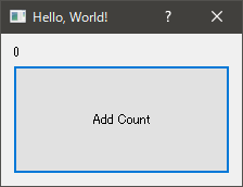
sample/gui.pyimport sys from PySide2 import QtCore from PySide2 import QtWidgets class SampleDialog(QtWidgets.QDialog): def __init__(self, *args): super(SampleDialog, self).__init__(*args) self.number = 0 self.setWindowTitle('Hello, World!') self.resize(300, 200) layout = QtWidgets.QVBoxLayout() self.label = QtWidgets.QLabel(str(self.number)) layout.addWidget(self.label) self.button = QtWidgets.QPushButton('Add Count') self.button.clicked.connect(self.add_count) self.button.setMinimumSize(200, 100) layout.addWidget(self.button) self.setLayout(layout) self.resize(200, 100) def add_count(self): self.number += 2 self.label.setText(str(self.number)) def main(): app = QtWidgets.QApplication.instance() if app is None: app = QtWidgets.QApplication(sys.argv) gui = SampleDialog() gui.show() app.exec_() if __name__ == '__main__': main()実行した際の見た目は、次の様になる。
requirements.txt に必要モジュールを書く
PySide2
Pytest
venv環境を作成する
- rootディレクトリに行く
python -m venv .venv- venv環境を有効にする:
.venv\Script\Activate.batpip install -r requirements.txtconftest.pyでモジュールへのパスをつなぐ
tests/conftest.pyimport os import sys sys.path.append(os.path.dirname(os.path.abspath(__file__)))Pytest公式では、setup.pyを用いた、
pip install -e .を使って、インストールする事が推奨されているが、TAの(DCCツールも含めた)ツールリリース環境の場合、必ずしもpip環境を提供するわけにはいかない場合がある。そういった場合に、余計なディレクトリ構成を取りたくない事があるので、conftest.pyを使用して、Pytestの実行じにrootにパスを通しておく。
もちろん、
pip installを前提とした配布環境の場合はpip intall -e .を出来るように、 setup.pyをroot下に配置し、pip install出来るようにしておくと良い。また、同様に、Mayaなどの外部ツールなどで必要なモジュールがあるみたいな時には、ここでパスを通しに行くと良い。
テストコードの実装
Pytestでのテストファイル
Pytestは、test_.py や *test.pyというファイルを検索して、自動で取得しにいく。
さらに、そのファイルの中のtestという関数を探して実行する。
さらに、その関数をまとめたい場合には、Test*(Ex: TestGui)といったクラスを作ると、これもまたPytestが自動で拾いに行ってくれる。テストを書いていく
tests/unit/test_gui.pyimport sys from PySide2 import QtCore from PySide2 import QtWidgets from PySide2 import QtTest def test_add_count(): from sample import gui app = QtWidgets.QApplication.instance() if app is None: app = QtWidgets.QApplication(sys.argv) gui = gui.SampleDialog() gui.show() QtTest.QTest.mouseClick(gui.button, QtCore.Qt.LeftButton) n1 = gui.number QtTest.QTest.mouseClick(gui.button, QtCore.Qt.LeftButton) n2 = gui.number assert abs(n2 - n1) == 1QtTestを使う
ここで出てくるのが、QtTestで、PySideはこうしてテスト用のモジュールを提供してくれている。
ユーザーは、「『ボタンをクリックすることによって』、ラベルの数字が1上がる」という事を認識するので、この動作が正しくなるように、『ボタンをクリックすることによって』というのをテスト上でシミュレートする必要がある。
ここでQtTestは、QtTest.QTest.mousClick()を使う事によって、その動作をシミュレートすることができるようになる。つまり、上記のtest_add_countでは、次のことをQtTestで行っている
- 最初のQtTest.QTest.mousClicke()で、「guiのボタンを左マウスクリックする」
- その時のnumberクラス変数の値をn1として格納する
- 次のQtTest.QTest.mousClicke()で、「guiのボタンを左マウスクリックする」
- 二回目のクリックした状態でのnumberクラス変数の値をn2として格納する
- assertでその二つの格納した値を比較し、差が1であることを確認する
これにより、 ボタンをクリックした際の変更が、正しくカウントの上昇が1づつであるということを保証することができる。
テストコマンドを実行する
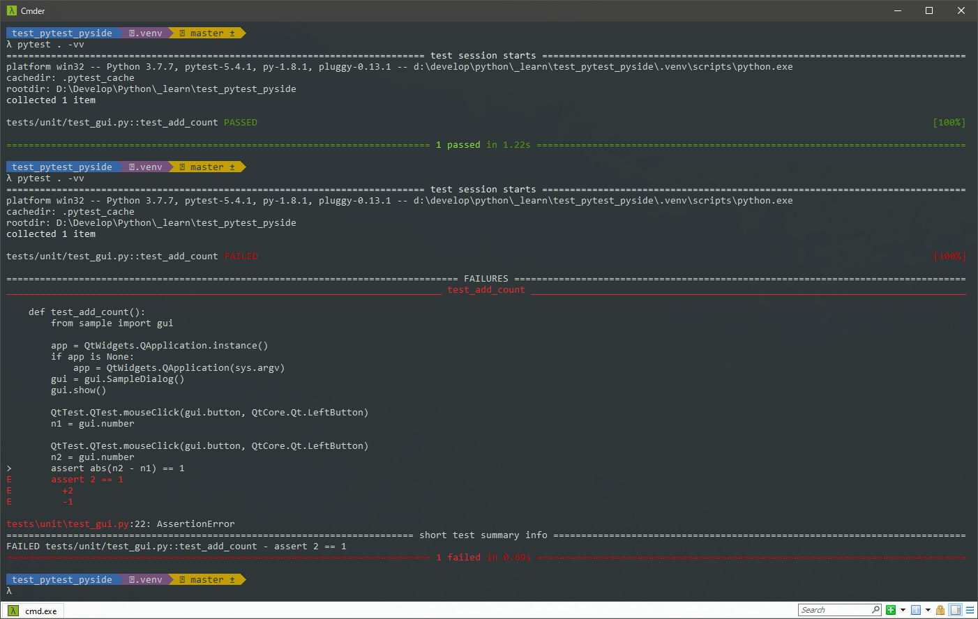
テストを実行する際のコマンドをルートディレクトリでとりあえずこれを実行すればいい。
pytest .すると、次の様な結果が得られる。
================================== test session starts ==================================
platform win32 -- Python 3.7.7, pytest-5.4.1, py-1.8.1, pluggy-0.13.1
rootdir: D:\Develop\Python\_learn\test_pytest_pyside
collected 1 item

F                                                           [100%]

======================================= FAILURES ========================================
____________________________________ test_add_count _____________________________________

    def test_add_count():
        from sample import gui

        app = QtWidgets.QApplication.instance()
        if app is None:
            app = QtWidgets.QApplication(sys.argv)
        gui = gui.SampleDialog()
        gui.show()

        QtTest.QTest.mouseClick(gui.button, QtCore.Qt.LeftButton)
        n1 = gui.number

        QtTest.QTest.mouseClick(gui.button, QtCore.Qt.LeftButton)
        n2 = gui.number
>       assert abs(n2 - n1) == 1
E       assert 2 == 1
E        +  where 2 = abs((4 - 2))

tests\unit\test_gui.py:22: AssertionError
================================ short test summary info ================================
FAILED tests/unit/test_gui.py::test_add_count - assert 2 == 1
=================================== 1 failed in 0.89s ===================================
これを説明すると、
テスト上のコードを見ての通り、add_countは、最初の実行と次の実行時の値の差が1であってほしいという開発者の意図がある。しかしながら、ソースコードを見てみると、self.number += 2としてあり、『ボタンをクリックすることによって』実行された処理の結果の差が2の結果を出してしまっている。では、この
self.number += 1に変え、「1づつ増える(つまり常に増える差は1)」にしてみると、pytest .を実行した際に、次の結果が得られる。================================== test session starts ================================== platform win32 -- Python 3.7.7, pytest-5.4.1, py-1.8.1, pluggy-0.13.1 rootdir: D:\Develop\Python\_learn\test_pytest_pyside collected 1 item . [100%] =================================== 1 passed in 1.44s ===================================この様にして、テストの成功の結果が得られた。
まとめ
Pytestは先のように、自動でテストコードを拾ってきたり、conftest.pyを使用することによって、あらかじめ前提としたい環境設定も用意することができるので、様々な排他的環境を少ないコードで、自動で構築できるようになる。
PySideは、QtTestという機能をあらかじめ用意しており、これを使用することでGuiの挙動をシミュレートできることがわかる。よくよく調べていくと、Pytestにももっともっと機能が豊富にあり、QtTestも同じく機能をたくさん持っているので、このスタートアップを経て、様々なテスト実装を行えて良ければと考える。
- 投稿日:2020-03-27T19:07:44+09:00
PySide & Pytest での テスト駆動開発 スタートアップ
はじめに
PySide勉強会での、「PySide & Pytest で テスト駆動開発スタートアップ」の補足記事。
および、PySideとPytestでテスト駆動開発をするためのメモ。
開発環境
Windows 10
Python 3.7.7
Pytestサンプルファイル
初期整備
ディレクトリとファイルの準備
ディレクトリroot |- sample | |- __init__.py | |- gui.py |- tests | |- __init__.py | |- conftest.py | |- unit | |- test_gui.py |- requirments.txtここでのツールのソースとなるgui.pyは以下のようなものを用意した。
sample/gui.pyimport sys from PySide2 import QtCore from PySide2 import QtWidgets class SampleDialog(QtWidgets.QDialog): def __init__(self, *args): super(SampleDialog, self).__init__(*args) self.number = 0 self.setWindowTitle('Hello, World!') self.resize(300, 200) layout = QtWidgets.QVBoxLayout() self.label = QtWidgets.QLabel(str(self.number)) layout.addWidget(self.label) self.button = QtWidgets.QPushButton('Add Count') self.button.clicked.connect(self.add_count) self.button.setMinimumSize(200, 100) layout.addWidget(self.button) self.setLayout(layout) self.resize(200, 100) def add_count(self): self.number += 2 self.label.setText(str(self.number)) def main(): app = QtWidgets.QApplication.instance() if app is None: app = QtWidgets.QApplication(sys.argv) gui = SampleDialog() gui.show() app.exec_() if __name__ == '__main__': main()実行した際の見た目は、次の様になる。
requirements.txt に必要モジュールを書く
PySide2
Pytest
venv環境を作成する
- rootディレクトリに行く
python -m venv .venv- venv環境を有効にする:
.venv\Script\Activate.batpip install -r requirements.txtconftest.pyでモジュールへのパスをつなぐ
tests/conftest.pyimport os import sys sys.path.append(os.path.dirname(os.path.abspath(__file__)))Pytest公式では、setup.pyを用いた、
pip install -e .を使って、インストールする事が推奨されているが、TAの(DCCツールも含めた)ツールリリース環境の場合、必ずしもpip環境を提供するわけにはいかない場合がある。そういった場合に、余計なディレクトリ構成を取りたくない事があるので、conftest.pyを使用して、Pytestの実行じにrootにパスを通しておく。
もちろん、
pip installを前提とした配布環境の場合はpip intall -e .を出来るように、 setup.pyをroot下に配置し、pip install出来るようにしておくと良い。また、同様に、Mayaなどの外部ツールなどで必要なモジュールがあるみたいな時には、ここでパスを通しに行くと良い。
テストコードの実装
Pytestでのテストファイル
Pytestは、test_.py や *test.pyというファイルを検索して、自動で取得しにいく。
さらに、そのファイルの中のtestという関数を探して実行する。
さらに、その関数をまとめたい場合には、Test*(Ex: TestGui)といったクラスを作ると、これもまたPytestが自動で拾いに行ってくれる。テストを書いていく
tests/unit/test_gui.pyimport sys from PySide2 import QtCore from PySide2 import QtWidgets from PySide2 import QtTest def test_add_count(): from sample import gui app = QtWidgets.QApplication.instance() if app is None: app = QtWidgets.QApplication(sys.argv) gui = gui.SampleDialog() gui.show() QtTest.QTest.mouseClick(gui.button, QtCore.Qt.LeftButton) n1 = gui.number QtTest.QTest.mouseClick(gui.button, QtCore.Qt.LeftButton) n2 = gui.number assert abs(n2 - n1) == 1QtTestを使う
ここで出てくるのが、QtTestで、PySideはこうしてテスト用のモジュールを提供してくれている。
ユーザーは、「『ボタンをクリックすることによって』、ラベルの数字が1上がる」という事を認識するので、この動作が正しくなるように、『ボタンをクリックすることによって』というのをテスト上でシミュレートする必要がある。
ここでQtTestは、QtTest.QTest.mousClick()を使う事によって、その動作をシミュレートすることができるようになる。つまり、上記のtest_add_countでは、次のことをQtTestで行っている
- 最初のQtTest.QTest.mousClicke()で、「guiのボタンを左マウスクリックする」
- その時のnumberクラス変数の値をn1として格納する
- 次のQtTest.QTest.mousClicke()で、「guiのボタンを左マウスクリックする」
- 二回目のクリックした状態でのnumberクラス変数の値をn2として格納する
- assertでその二つの格納した値を比較し、差が1であることを確認する
これにより、 ボタンをクリックした際の変更が、正しくカウントの上昇が1づつであるということを保証することができる。
テストコマンドを実行する
テストを実行する際のコマンドをルートディレクトリでとりあえずこれを実行すればいい。
pytest .すると、次の様な結果が得られる。
======================================= test session starts ========================================
platform win32 -- Python 3.7.7, pytest-5.4.1, py-1.8.1, pluggy-0.13.1
rootdir: D:\Develop\Python\_learn\test_pytest_pyside
collected 1 item

tests\unit\test_gui.py F                                                                      [100%]

============================================= FAILURES =============================================
__________________________________________ test_add_count __________________________________________

    def test_add_count():
        from sample import gui

        app = QtWidgets.QApplication.instance()
        if app is None:
            app = QtWidgets.QApplication(sys.argv)
        gui = gui.SampleDialog()
        gui.show()

        QtTest.QTest.mouseClick(gui.button, QtCore.Qt.LeftButton)
        n1 = gui.number

        QtTest.QTest.mouseClick(gui.button, QtCore.Qt.LeftButton)
        n2 = gui.number
>       assert abs(n2 - n1) == 1
E       assert 2 == 1
E        +  where 2 = abs((4 - 2))

tests\unit\test_gui.py:22: AssertionError
===================================== short test summary info ======================================
FAILED tests/unit/test_gui.py::test_add_count - assert 2 == 1
======================================== 1 failed in 0.67s =========================================
これを説明すると、
テスト上のコードを見ての通り、add_countは、最初の実行と次の実行時の値の差が1であってほしいという開発者の意図がある。しかしながら、ソースコードを見てみると、self.number += 2としてあり、『ボタンをクリックすることによって』実行された処理の結果の差が2の結果を出してしまっている。では、この
self.number += 1に変え、「1づつ増える(つまり常に増える差は1)」にしてみると、pytest .を実行した際に、次の結果が得られる。======================================= test session starts ======================================== platform win32 -- Python 3.7.7, pytest-5.4.1, py-1.8.1, pluggy-0.13.1 rootdir: D:\Develop\Python\_learn\test_pytest_pyside collected 1 item tests\unit\test_gui.py . [100%] ======================================== 1 passed in 0.70s =========================================この様にして、テストの成功の結果が得られた。
まとめ
Pytestは先のように、自動でテストコードを拾ってきたり、conftest.pyを使用することによって、あらかじめ前提としたい環境設定も用意することができるので、様々な排他的環境を少ないコードで、自動で構築できるようになる。
PySideは、QtTestという機能をあらかじめ用意しており、これを使用することでGuiの挙動をシミュレートできることがわかる。よくよく調べていくと、Pytestにももっともっと機能が豊富にあり、QtTestも同じく機能をたくさん持っているので、このスタートアップを経て、様々なテスト実装を行えて良ければと考える。
- 投稿日:2020-03-27T19:02:10+09:00
AtCoder Beginner Contest 084 過去問復習
所要時間
感想
FXが今日は惨敗していて萎えてます。相場は巻き返さないし週末は東京封鎖だし最悪ですね。
今回は難しくないのですが、エラトステネスの篩をバグらせました。生きるのがしんどい。A問題
引き算、特に感想なし。
answerA.pyprint(48-int(input()))B問題
一文字ずつチェックします。
0~9の文字列を作ってその中にあるかで計算しましたが、"0"以上"9"以下としてもOKなようです。answerB.pynum=list("0123456789") a,b=map(int,input().split()) s=input() for i in range(a+b+1): if i!=a: if s[i] not in num: print("No") break else: if s[i]!="-": print("No") break else: print("Yes")C問題
頭が弱すぎて何回もミスりました。
それぞれの駅に何時に着くかをnowという変数に記録しておきます。そして、それぞれの駅についてはs以降かつその駅についた時間以降で最も小さいfの倍数を考えてそこからcだけ進めば次の駅に進むというのをまずは文字に起こして冷静に式を立てることで解けます。
僕はこれがFXの考えすぎでできませんでした。なんて頭が悪いんでしょうか。answerC.pyimport math n=int(input()) csf=[list(map(int,input().split())) for i in range(n-1)] for j in range(n-1): now=0 for i in range(j,n-1): if csf[i][1]>=now: now=csf[i][1]+csf[i][0] else: now=csf[i][1]-((csf[i][1]-now)//csf[i][2])*csf[i][2]+csf[i][0] print(now) print(0)D問題
区間のクエリが与えられてるので累積和の差を考えれば良いのは明らかです。
つまり、クエリの計算を行う前に"2017に似た数"を先に求めておけば良く、エラトステネスの篩(他記事で紹介しています。)を用いて素数列挙してから"2017に似た数"をチェックし、累積和を考えておけば良いです。
しかし、エラトステネスの篩がバグっていた上に"2017に似た数"をチェックするつもりが、ただ素数をチェックしたために時間がかかってしまいました。こういうケアレスミスを無くすようにしたいです。answerD.cc#include<algorithm>//sort,二分探索,など #include<bitset>//固定長bit集合 #include<cmath>//pow,logなど #include<complex>//複素数 #include<deque>//両端アクセスのキュー #include<functional>//sortのgreater #include<iomanip>//setprecision(浮動小数点の出力の誤差) #include<iostream>//入出力 #include<map>//map(辞書) #include<numeric>//iota(整数列の生成),gcdとlcm(c++17) #include<queue>//キュー #include<set>//集合 #include<stack>//スタック #include<string>//文字列 #include<unordered_map>//イテレータあるけど順序保持しないmap #include<unordered_set>//イテレータあるけど順序保持しないset #include<utility>//pair #include<vector>//可変長配列 using namespace std; typedef long long ll; //マクロ #define REP(i,n) for(ll i=0;i<(ll)(n);i++) #define REPD(i,n) for(ll i=(ll)(n)-1;i>=0;i--) #define FOR(i,a,b) for(ll i=(a);i<=(b);i++) #define FORD(i,a,b) for(ll i=(a);i>=(b);i--) #define ALL(x) (x).begin(),(x).end() //sortなどの引数を省略したい #define SIZE(x) ((ll)(x).size()) //sizeをsize_tからllに直しておく #define MAX(x) *max_element(ALL(x)) #define INF 1000000000000 #define MOD 10000007 #define MA 100000 #define PB push_back #define MP make_pair #define F first #define S second ll sieve_check[MA+1];//i番目が整数iに対応(1~100000) //エラトステネスの篩を実装する void es(){ FOR(i,2,MA)sieve_check[i]=1; //1のところが素数、ここでは0が素数でない for(ll i=2;i<=1000;i++){ if(sieve_check[i]==1){ for(ll j=2;j<=ll(MA/i);j++){ sieve_check[j*i]=0; } } } } signed main(){ es(); vector<ll> pre(MA+1);FOR(i,1,MA)pre[i]=(i%2==1&&sieve_check[i]&&sieve_check[(i+1)/2]); REP(i,MA)pre[i+1]+=pre[i]; ll q;cin >> q; vector< pair<ll,ll> > ans(q);REP(i,q) cin >> ans[i].F >> ans[i].S; REP(i,q)cout << pre[ans[i].S]-pre[ans[i].F-1] << endl; }

- 投稿日:2020-03-27T18:34:03+09:00
【python】pandasのread_html読み込みエラーの対処法
【python】pandasのread_html読み込みエラーの対処法
pandasの「read_html」というメソッドでhtmlファイルも読み込めるのか!と思い、試したところ連続で別々のエラーが、、
▼4つの課題(エラー)
①「ImportError: lxml not found, please install it」②「ImportError: html5lib not found, please install it」
③「ImportError: BeautifulSoup4 (bs4) not found, please install it」
④「ValueError: No tables found」
▼対応ポイント
・使うためにはライブラリをいくつかインストールしておく必要がある。・データ取得は表(テーブル)に対してのみ。
■対処法実例
下記3つのライブラリをインストールしてから、
表を含むページを指定して実行すればできます。①ライブラリのインストール
ライブラリのインストールpip install lxml pip install html5lib pip install bs4②データ取得実行
データ取得実行import pandas as pd url = 'https://stocks.finance.yahoo.co.jp/stocks/detail/?code=998407.O' df = pd.read_html(url)URL:日経平均株価【998407】:国内指数 - Yahoo!ファイナンス
無事取得できました。
補足
▼なぜ3つもインストールする必要があるのか
ページの解析はBeautifulSoup4で行う。その際、テーブルの解析にlxmlを使用。
lxmlでhtmlの解析に失敗した場合に、html5libを使用する。html5libは解析能力に優れ、htmlの補完もできるが重い。
ただし、html5libもインストールすることが推奨されている。
▼read_htmlでできること
要素のみにしか使えない。
子要素の、、 、 、。
■エラー詳細
第1のエラー
エラーimport pandas as pd url = 'https://www.yahoo.co.jp/' df = pd.read_html(url) #出力 # ImportError: lxml not found, please install itlxmlがインストールされていないとのこと。
lxmlとは?
pythonのライブラリの一種で、htmlやxmlを解析するもの。
非常に軽い。ただし、厳密なマークアップにしか対応していないため、解析に失敗することがある。
lxmlのインストール
pip install lxml第2のエラー
html5libとは?
lxmlを無事インストールし、再度実行したところ別のエラーが、、
「ImportError: html5lib not found, please install it」
こちらはhtml5を解析するもの。
lxmlよりも高性能。無効なマークアップから正しいマークアップを自動生成できる。その代わり重い。
lxmlでhtmlの解析に失敗した場合に、使われる。
html5libのインストール
pip install html5lib
第3のエラー
BeautifulSoup4 (bs4) とは?
html5libを無事インストールし、再度コードを実行したところ、新たなエラーが、、
「ImportError: BeautifulSoup4 (bs4) not found, please install it」
BeautifulSoup4 (bs4) はhtmlやxmlを解析するもの。
ページ解析の大本となるライブラリ。
今回のテーブルの解析には、バックエンドでlxmlやhtml5libが使われる。BeautifulSoup4 (bs4) のインストール
pip install bs4第4のエラー
bs4を無事インストールし、再度コードを実行したところ、新たなエラーが、、
「ValueError: No tables found」
どうやら表データしかとってこれないらしい。。
表データの取得
表データがあるサイトとして、yahooファイナンスの日経平均株価【998407】ページでトライ。
https://m.finance.yahoo.co.jp/stock?code=998407.O
read_htmlimport pandas as pd url = 'https://stocks.finance.yahoo.co.jp/stocks/detail/?code=998407.O' df = pd.read_html(url) df
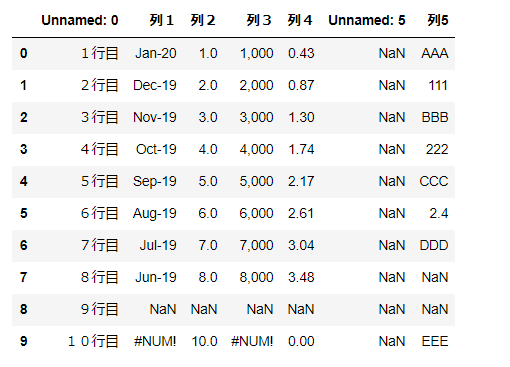
出力結果を見る
[        0   1         2                   3
 0  日経平均株価 NaN  19389.43  前日比+724.83(+3.88%),
       0             1
 0  株価予想  どうなる?明日の日経平均,
               0         1
 0        日経平均株価      NYダウ
 1         TOPIX   ナスダック総合
 2  ジャスダックインデックス   S&P 500
 3        香港ハンセン  FTSE 100
 4          上海総合       DAX
 5  ムンバイSENSEX30    CAC 40,
                                              0  \
 0                ピクテ・ゴールド(H有)その他リターン(1年)19.94%
 1              グローバルSDGs株式ファンドその他リターン(1年)5.27%
 2  eMAXIS Slim全世界株式(オール・カントリー)その他リターン(1年)3.91%

                                       1
 0  パインブリッジ・キャピタル証券F(H有)その他リターン(1年)6.35%
 1   リスクコントロール世界資産分散ファンドその他リターン(1年)4.81%
 2     米国株式配当貴族(年4回決算型)国際株式リターン(1年)2.21%  ,
                                                    0  \
 0  総合 値上がり率 1. 新都HLD+45.45% 2. スガイ化+28.30% 3. アマガ...

                                                    1
 0  東証1部 値上がり率 1. カネコ種+19.95% 2. セグエG+18.28% 3. 小林...  ]
- 投稿日:2020-03-27T17:44:55+09:00
Python未経験者が言語処理100本ノックをやってみる14~16
真面目に仕事をしていると投稿をサボることになり、
真面目に投稿していると仕事をサボることになる。これは難しい問題だ・・・(真剣)
(休みの日はやらん)これの続きでーす。
Python未経験者が言語処理100本ノックをやってみる10~13
https://qiita.com/earlgrey914/items/afdb6458a2c9f1c00c2e
14. 先頭からN行を出力
自然数Nをコマンドライン引数などの手段で受け取り,入力のうち先頭のN行だけを表示せよ.確認にはheadコマンドを用いよ.
コマンドライン引数を得るには以下のように書けばいいらしい。
arg.pyimport sys args = sys.argv<参考URL>
https://qiita.com/orange_u/items/3f0fb6044fd5ee2c3a37args[1]とインデックスが1から始まっているのは,実行結果を見れば理由が分かる
実行結果からわかるように,リストとして値が返されるふむふむ。コマンドライン引数はリストとして返され、1からカウントと。
えーと、問題文が少し難解だけど、「2」がコマンドライン引数で渡されたら
merge.txtの2行を出力すればいいってことかしらね。これでどうでしょ。
otto.pyimport os.path import sys os.chdir((os.path.dirname(os.path.abspath(__file__)))) args = sys.argv linedata = [] with open('merge.txt', mode="r") as f: linedata = f.read().splitlines() print(linedata[args[1])])[ec2-user@ip-172-31-34-215 02]$ python3 enshu14.py 2 Traceback (most recent call last): File "enshu14.py", line 11, in <module> print(linedata[args[1]]) TypeError: list indices must be integers or slices, not strおっと、コマンドライン引数
argsのリストは文字列で返されるようだ。入力値は文字列型として扱われる
では文字列→整数変換を。
int(args[1])ですねenshu14.pyimport os.path import sys os.chdir((os.path.dirname(os.path.abspath(__file__)))) args = sys.argv linedata = [] with open('merge.txt', mode="r") as f: linedata = f.read().splitlines() for i in range(int(args[1])): print(linedata[i])引数を2とか5にしてみて検証。
[ec2-user@ip-172-31-34-215 02]$ python3 enshu14.py 2
高知県  江川崎
埼玉県  熊谷
[ec2-user@ip-172-31-34-215 02]$ python3 enshu14.py 5
高知県  江川崎
埼玉県  熊谷
岐阜県  多治見
山形県  山形
山梨県  甲府
[ec2-user@ip-172-31-34-215 02]$
うーん簡単。
headとも比較。[ec2-user@ip-172-31-34-215 02]$ head -n 2 merge.txt 高知県 江川崎 埼玉県 熊谷 [ec2-user@ip-172-31-34-215 02]$ head -n 5 merge.txt 高知県 江川崎 埼玉県 熊谷 岐阜県 多治見 山形県 山形 山梨県 甲府 [ec2-user@ip-172-31-34-215 02]$~5日ほどサボり~
末尾のN行を出力
自然数Nをコマンドライン引数などの手段で受け取り,入力のうち末尾のN行だけを表示せよ.確認にはtailコマンドを用いよ.
リストを末尾から参照するには
[-1]、[-2]、[-3]、・・・と参照していけば良いらしい。<参考URL>
https://qiita.com/komeiy/items/971ead35d33c25923222これ出力結果はどうなればいいんだ?
["a", "b", "c", "d"]のリストがあって、引数が2ならc, dと出力されればいいのか?d, cなのか?
tailで確認せよとのことなので、まずtailだとどう出力されるか確認してみよう。[ec2-user@ip-172-31-34-215 02]$ tail -n 2 merge.txt 山形県 鶴岡 愛知県 名古屋 [ec2-user@ip-172-31-34-215 02]$ tail -n 5 merge.txt 埼玉県 鳩山 大阪府 豊中 山梨県 大月 山形県 鶴岡 愛知県 名古屋なるほど。
c, dの順で出せば良いんだな。enshu15.pyimport os.path import sys os.chdir((os.path.dirname(os.path.abspath(__file__)))) args = sys.argv linedata = [] with open('merge.txt', mode="r") as f: linedata = f.read().splitlines() linedata_reverse =[] for i in range(int(args[1])): linedata_reverse.append(linedata[-i-1]) for i in (reversed(linedata_reverse)): print(i)うい。できました。
リストの反転はreversed()ですね。[ec2-user@ip-172-31-34-215 02]$ python3 enshu15.py 2 山形県 鶴岡 愛知県 名古屋 [ec2-user@ip-172-31-34-215 02]$ python3 enshu15.py 5 埼玉県 鳩山 大阪府 豊中 山梨県 大月 山形県 鶴岡 愛知県 名古屋結果もOK。
Pythonってこういうリストの反転とかスライスとか、便利な標準機能が多いなーって感じます。
16. ファイルをN分割する
自然数Nをコマンドライン引数などの手段で受け取り,入力のファイルを行単位でN分割せよ.同様の処理をsplitコマンドで実現せよ.
まずは
splitコマンドがどのようなものか試してみる。
お気づきかと思うが、筆者はPythonも初心者だし、UNIXコマンドも初心者である。[ec2-user@ip-172-31-34-215 02]$ split -l 2 -d merge.txt test [ec2-user@ip-172-31-34-215 02]$ ll total 112 -rw-rw-r-- 1 ec2-user ec2-user 435 Mar 19 17:12 merge.txt -rw-rw-r-- 1 ec2-user ec2-user 37 Mar 25 15:48 test00 -rw-rw-r-- 1 ec2-user ec2-user 37 Mar 25 15:48 test01 -rw-rw-r-- 1 ec2-user ec2-user 43 Mar 25 15:48 test02 -rw-rw-r-- 1 ec2-user ec2-user 34 Mar 25 15:48 test03 -rw-rw-r-- 1 ec2-user ec2-user 34 Mar 25 15:48 test04 -rw-rw-r-- 1 ec2-user ec2-user 37 Mar 25 15:48 test05 -rw-rw-r-- 1 ec2-user ec2-user 37 Mar 25 15:48 test06 -rw-rw-r-- 1 ec2-user ec2-user 37 Mar 25 15:48 test07 -rw-rw-r-- 1 ec2-user ec2-user 34 Mar 25 15:48 test08 -rw-rw-r-- 1 ec2-user ec2-user 34 Mar 25 15:48 test09 -rw-rw-r-- 1 ec2-user ec2-user 34 Mar 25 15:48 test10 -rw-rw-r-- 1 ec2-user ec2-user 37 Mar 25 15:48 test11 [ec2-user@ip-172-31-34-215 02]$ cat test00 高知県 江川崎 埼玉県 熊谷なるほど。
ではまず、「行単位でN分割」の部分を作ろう。enshu16.pyimport os.path import sys os.chdir((os.path.dirname(os.path.abspath(__file__)))) args = sys.argv a = int(args[1]) linedata = [] with open('merge.txt', mode="r") as f: linedata = f.read().splitlines() for i in range(0, len(linedata), a): print(linedata[i:i+a:])とりあえずこれで、リストを分割したかのように表示することができた。
[ec2-user@ip-172-31-34-215 02]$ python3 enshu16.py 1
['高知県\t江川崎']
['埼玉県\t熊谷']
['岐阜県\t多治見']
['山形県\t山形']
['山梨県\t甲府']
['和歌山県\tかつらぎ']
['静岡県\t天竜']
['山梨県\t勝沼']
['埼玉県\t越谷']
['群馬県\t館林']
['群馬県\t上里見']
['愛知県\t愛西']
['千葉県\t牛久']
['静岡県\t佐久間']
['愛媛県\t宇和島']
['山形県\t酒田']
['岐阜県\t美濃']
['群馬県\t前橋']
['千葉県\t茂原']
['埼玉県\t鳩山']
['大阪府\t豊中']
['山梨県\t大月']
['山形県\t鶴岡']
['愛知県\t名古屋']
[ec2-user@ip-172-31-34-215 02]$ python3 enshu16.py 2
['高知県\t江川崎', '埼玉県\t熊谷']
['岐阜県\t多治見', '山形県\t山形']
['山梨県\t甲府', '和歌山県\tかつらぎ']
['静岡県\t天竜', '山梨県\t勝沼']
['埼玉県\t越谷', '群馬県\t館林']
['群馬県\t上里見', '愛知県\t愛西']
['千葉県\t牛久', '静岡県\t佐久間']
['愛媛県\t宇和島', '山形県\t酒田']
['岐阜県\t美濃', '群馬県\t前橋']
['千葉県\t茂原', '埼玉県\t鳩山']
['大阪府\t豊中', '山梨県\t大月']
['山形県\t鶴岡', '愛知県\t名古屋']
[ec2-user@ip-172-31-34-215 02]$ python3 enshu16.py 5
['高知県\t江川崎', '埼玉県\t熊谷', '岐阜県\t多治見', '山形県\t山形', '山梨県\t甲府']
['和歌山県\tかつらぎ', '静岡県\t天竜', '山梨県\t勝沼', '埼玉県\t越谷', '群馬県\t館林']
['群馬県\t上里見', '愛知県\t愛西', '千葉県\t牛久', '静岡県\t佐久間', '愛媛県\t宇和島']
['山形県\t酒田', '岐阜県\t美濃', '群馬県\t前橋', '千葉県\t茂原', '埼玉県\t鳩山']
['大阪府\t豊中', '山梨県\t大月', '山形県\t鶴岡', '愛知県\t名古屋']
次はファイルへの保存だ。
この問題では、元ファイルを 第2引数の名前+通番 の名前のファイルに分割する必要がある。
どうすればいいんだろう?~10分ほどググる~
<参考URL>
https://news.mynavi.jp/article/zeropython-40/なんかこういうふうに書けば連番ファイルの保存ができそう。
kou.pyfor i in range(5): print("テスト-{0:03d}.jpg".format(i + 1))テスト-001.jpg テスト-002.jpg テスト-003.jpg テスト-004.jpg テスト-005.jpg
format()というものを使うようだ。
個人的にものすごく難しく感じる。なんでダブルクオーテーションで囲った文字に直接.format()をつけて、値を渡せるんだ・・・?
{}の書き方のおかげだと思うんだけどこれなんて記法?~5分ほどググる~
うーん、なんだかシックリこないなー。
別にformat()を使わずとも他の書き方でもいけるようだし、他の書き方を使おう。
よくわからんものを「動くから」と使っていると後からさらによくわからんことになる。経験則です。<参考URL>
https://gammasoft.jp/blog/python-string-format/書き直し↓
tes.pyfor i in range(3): with open("テスト"+ str(i+1) +".txt", 'a') as f: print("てすと", file=f )[ec2-user@ip-172-31-34-215 02]$ ll total 124 -rw-rw-r-- 1 ec2-user ec2-user 3 Mar 27 17:15 テスト1.txt -rw-rw-r-- 1 ec2-user ec2-user 3 Mar 27 17:15 テスト2.txt -rw-rw-r-- 1 ec2-user ec2-user 3 Mar 27 17:15 テスト3.txtよし、これで良い。単に連結演算子を使えばいいだけだった。
ダサいかもしれないけど、俺にとっては一番わかりやすい。では課題の回答を作成。
enshu16.pyimport os.path import sys os.chdir((os.path.dirname(os.path.abspath(__file__)))) args = int(sys.argv[1]) linedata = [] with open('merge.txt', mode="r") as f: linedata = f.read().splitlines() for i in range(0, len(linedata), args): with open("テスト"+ str(i+1) +".txt", 'a') as f: output = linedata[i:i+args:] for j in output: print(j, file =f)[ec2-user@ip-172-31-34-215 02]$ python3 enshu16.py 2 [ec2-user@ip-172-31-34-215 02]$ ll total 160 -rw-rw-r-- 1 ec2-user ec2-user 37 Mar 27 17:30 テスト11.txt -rw-rw-r-- 1 ec2-user ec2-user 37 Mar 27 17:30 テスト13.txt -rw-rw-r-- 1 ec2-user ec2-user 37 Mar 27 17:30 テスト15.txt -rw-rw-r-- 1 ec2-user ec2-user 34 Mar 27 17:30 テスト17.txt -rw-rw-r-- 1 ec2-user ec2-user 34 Mar 27 17:30 テスト19.txt -rw-rw-r-- 1 ec2-user ec2-user 37 Mar 27 17:30 テスト1.txt -rw-rw-r-- 1 ec2-user ec2-user 34 Mar 27 17:30 テスト21.txt -rw-rw-r-- 1 ec2-user ec2-user 37 Mar 27 17:30 テスト23.txt -rw-rw-r-- 1 ec2-user ec2-user 37 Mar 27 17:30 テスト3.txt -rw-rw-r-- 1 ec2-user ec2-user 43 Mar 27 17:30 テスト5.txt -rw-rw-r-- 1 ec2-user ec2-user 34 Mar 27 17:30 テスト7.txt -rw-rw-r-- 1 ec2-user ec2-user 34 Mar 27 17:30 テスト9.txt -rw-rw-r-- 1 ec2-user ec2-user 530 Mar 27 17:29 enshu16.py -rw-rw-r-- 1 ec2-user ec2-user 435 Mar 19 17:12 merge.txt [ec2-user@ip-172-31-34-215 02]$ cat テスト1.txt 高知県 江川崎 埼玉県 熊谷できたぞー。
通番を0埋めしていないから並び順が無茶苦茶ね。
通番を0埋めするときは多分format()が役に立つんだろうな、と気づきました。
今回は使わないけどそのうち使います。ここまで多分3時間くらいかかりました!!!!!!!!
2章はわりと簡単ですね。あとqiita投稿に慣れてきて、逆にやる気がなくなってきたせいでダラダラやってます。
- 投稿日:2020-03-27T17:12:57+09:00
SQLite3を簡単に使ってみる
SQLiteは,小規模なデータベースをサクっと作りたいときに使われるデータベースマネジメントシステム(DBMS)のひとつです.
データベースとは
データを登録したり,削除したり,検索したりするシステムのこと.
参照:データベースのきほん
いまさら聞けないデータベースとは?データベースの種類
- MySQL
- PostgreSQL
- SQLite
- Oracle DB
などがあります.(参照:MySQL、PostgreSQL、SQLite、Oracle DBの比較)
中でも,SQLite3はPythonの標準ライブラリに既に入っていて,機能が少なく,手軽に使えます.
SQLite3の使い方
pythonとは別に,SQLを書く必要があります.
#インポート
import sqlite3

#データベースに接続
filepath = "test2.sqlite"
conn = sqlite3.connect(filepath)
#filepathと同名のファイルがなければ,ファイルが作成されます

#テーブルを作成
cur = conn.cursor()
cur.execute("DROP TABLE IF EXISTS items")

cur.execute("""CREATE TABLE items(
    item_id INTEGER PRIMARY KEY,
    name TEXT UNIQUE,
    price INTEGER
)""")
conn.commit()

#単発でデータを挿入
cur.execute('INSERT INTO items (name , price) VALUES (?,?)',("Orange", 520))
conn.commit()

#連続でデータを挿入
cur = conn.cursor()
data = [("Mango",770),("Kiwi", 400), ("Grape",800),("Peach",940),("Persimmon",700), ("Banana",400)]
cur.executemany(
    "INSERT INTO items (name, price) VALUES (?,?)", data)
conn.commit()
以上でデータベースの構築と,データの登録ができました.
conn.commit()を実行しないと,データベースにコマンドが反映されないことに注意.全データを表示してみます.
#全データを抽出する
cur = conn.cursor()
cur.execute("SELECT item_id, name, price FROM items")
items_list = cur.fetchall()
items_list
[(1, 'Orange', 520), (2, 'Mango', 770), (3, 'Kiwi', 400), (4, 'Grape', 800), (5, 'Peach', 940), (6, 'Persimmon', 700), (7, 'Banana', 400)]for文で1つずつ表示してみます.
#全データを抽出する(for文使用)
cur = conn.cursor()
cur.execute("SELECT item_id, name, price FROM items")
items_list = cur.fetchall()
for fr in items_list:
    print(fr)
(1, 'Orange', 520) (2, 'Mango', 770) (3, 'Kiwi', 400) (4, 'Grape', 800) (5, 'Peach', 940) (6, 'Persimmon', 700) (7, 'Banana', 400)検索をかけてみます.
#400-700円のデータを抽出して表示
cur = conn.cursor()
price_range = (400, 700)
cur.execute(
    "SELECT * FROM items WHERE price >=? AND PRICE <=?", price_range
)
fr_list = cur.fetchall()
for fr in fr_list:
    print(fr)
(1, 'Orange', 520) (3, 'Kiwi', 400) (6, 'Persimmon', 700) (7, 'Banana', 400)以上
- 投稿日:2020-03-27T17:10:53+09:00
【python】csvファイルの読み込みを使いこなす。pandas.read_csvの主要オプション一覧。
【python】csvファイルの読み込みを使いこなす。pandas.read_csvの主要オプション一覧。
pandasでのcsvファイルの読み込みの応用編
読み込む行・列の指定など、思っていた以上にできることが多いのでメモ。基本的にはこれだけ押さえておけばOK
read_csvメソッドの主要オプション一覧
・pythonでのcsvファイル読み込みの基本編はこちら
・公式ページはこちら
目次
- read_csvメソッドの主要オプション一覧
- デフォルトで読み込んだデータ
- 元ファイルの空白行・列・セル
- ヘッダー
- 見出し列(インデックス)の指定
- 列の読み込み
- 行の読み込み
- 型を指定して読み込む
- WEB上のファイルの読み込み
- 圧縮ファイルの読み込み
- 区切り文字を指定して読み込み
1. read_csvメソッドの主要オプション一覧
オプション 使用例 内容 sep sep=';' 分割(separate) delimiter delimiter=';' 分割(sepと同じ) header header=1 ヘッダー行の指定(デフォルトは推測、ない場合 header=None ※「N」は大文字) names ①names=['AA','BB','CC',,] ②names='1234567' 列タイトルを付ける(ヘッダーがある場合は「header=0」と併用) index_col index_col=0 行の見出し(index)となる列を指定 usecols usecols=[1,2,5] 読み込む行を指定。1行のみでもリスト形式で指定「usecols=[0]。列タイトルでも指定可能」 prefix prefix="行番号", header=None 行タイトルの接頭語を指定。例「prefix='行番号'」なら行番号0、行番号1、、、となる。 hedar=Noneを指定したときのみ有効。 dtype dtype=str 型を指定して読み込み。適用できない場合はエラー(strをfloatで読み込むなど) skiprows ①skiprows=5 ②skiprows=[1,3,6] 冒頭で読み込まない行番号を指定。整数の場合は0から指定した整数まで。 skipfooter skipfooter=2, engine='python', encoding='utf_8' 下から除外する行数を指定。pythonで使うことを記述する必要あり。文字化けする場合は文字コードを指定。 nrows nrows=5 何行目まで読み込むかを指定。 encoding encoding='shift_jis' ファイル読み込み時の文字コード指定 (compression) compression='zip' 圧縮ファイルを開く。現状、記述しなくても類推して開いてくれる。(逆にzipファイルにcompression='gzip'を指定するとエラー) (skipinitialspace) skipinitialspace=True デリミタ(文字区切り)後に、先頭についている空白を削除する。現状、デフォルトで削除される仕様のよう
2. デフォルトで読み込んだデータ
■元ファイル
以下のようなcsvファイル読み込んだ場合
▼列
・A列がindex(見出し)
・F列が空
・G列が文字と空白セル▼行
・1行目が列のタイトル
・9行目が空
・10行目に数式エラー(#NUM!)がある
■読み込み結果
▼ポイント
・1列目に見出し列が追加(0からのindex番号)
・1行目にタイトル行が追加
- 空白のセルは「Unnamed:列番号」で補完
・空白セルはNaNになる。
・数式エラーは #NUM!のまま表示される。※追加内容は再度ファイルに出力する場合に残る。(NaNは消える)
■各列の属性
列の属性Unnamed: 0 object 列1 object 列2 float64 列3 object 列4 float64 Unnamed: 5 float64 列5 object・日付:object型
・数値:float64型
└ 整数・少数どちらも
└ NaNは無視される
・関数エラーがある列:object型
・空の列:float64型
・テキスト:object型
└ テキストセルが1個あればobject型になる
■読み込み結果を出力
utf8でcsvファイルとして出力した場合。
・1行目と1列目に自動挿入された見出しは残る。
・NaNは空白行になる
3. 元ファイルの空白行・列・セル
空白は「NaN」(空データ)として処理される。
下記もNaNとして扱われる。
- 「''」
- 「#N/A」
- 「#N/A N/A」
- 「#NA」
- 「-1.#IND」
- 「-1.#QNAN」
- 「-NaN」
- 「-nan」
- 「1.#IND」
- 「1.#QNAN」
- 「」
- 「N/A」
- 「NA」
- 「NULL」
- 「NaN」
- 「n/a」
- 「nan」
- 「null」
4. ヘッダー
読み込み時デフォルトは「類推」となっている。
※基本的に最上部の行がヘッダーとして読み込まれる。▼元ファイル
▼読み込み結果
csvファイル読み込みimport pandas as pd df = pd.read_csv('~/desktop/test.csv') df└ デスクトップのtest.csvファイルを読み込み、表示。
①ヘッダーがないファイルの読み込み
オプションでヘッダーがないことを指定する。
header=None▼元ファイル(「デスクトップのtest2.csv」とする)
▼読み込みファイル
pd.read_csv('~/desktop/test2.csv' ,header=None)
import pandas as pd df = pd.read_csv('~/desktop/test2.csv' ,header=None) df※NoneのNは大文字。(noneはエラー)
▼指定がない場合
df2 = pd.read_csv('~/desktop/test2.csv')
②ヘッダーとなる行を指定する
※指定した行より上は読み込まれない。
▼ヘッダーとなる行を指定した場合
オプションで
header=整数を記述import pandas as pd df = pd.read_csv('~/desktop/test.csv' ,header=6) df
▼指定しない場合
③ヘッダー名を指定して読み込む
オプションで
names=を記述。
書き方は2種類。(1)連続した文字列
(2)list形式▼ポイント
・既にheaderがある場合は、header=0で上書きする。
・読み込む列数より指定文字数が少ない場合:先方の列タイトルは空白
・指定文字数の方が多い場合:後方の列タイトルはNaN
・異なる列に同じ名前は付けられない(エラー)
■実例(7列あるデータで実行結果を試す)
(1)連続した文字列で指定
▼例1:
names='123345'の場合import pandas as pd df = pd.read_csv('~/desktop/test.csv' ,names='12345') df
先頭の足りない2列分が空白となる。
▼例2:names='abcdefghi'の場合import pandas as pd df = pd.read_csv('~/desktop/test.csv' ,names='abcdefghi') df
多い列タイトル分は中身が空(NaN)の列となる。
▼例3:names='aaabbbccc'重複する場合はエラーimport pandas as pd df = pd.read_csv('~/desktop/test.csv' ,names='aaabbbccc') df #出力 # ValueError: Duplicate names are not allowed.
(2)list形式で指定
▼例1:
names=['aaa','bbb','ccc','ddd','eee','fff']の場合import pandas as pd df = pd.read_csv('~/desktop/test.csv' ,names=['aaa','bbb','ccc','ddd','eee','fff']) df
▼例2:names=['aaa','bbb','aaa','ddd']重複はエラーimport pandas as pd df = pd.read_csv('~/desktop/test.csv' ,names=['aaa','bbb','aaa','ddd']) df
ヘッダー名に共通の接頭語を指定する
prefix='文字列', header=None
└ header=Noneの場合のみ有効(ないときは無視される)
└ 指定した文字列に列番号がつく。
import pandas as pd df = pd.read_csv('~/desktop/test.csv', prefix="XXX", header=None) df
5. 見出し列(インデックス)の指定
オプションに
index_col=整数を記述。
デフォルトは自動でインデックス番号が振られた列が追加される。
python
import pandas as pd
df = pd.read_csv('~/desktop/test.csv' ,index_col=0)
df
デフォルト(指定なし)の場合
6. 列の読み込み
列番号または列名で指定できる。
①列番号で指定
②列名で指定
▼元ファイルは下記を使用
import pandas as pd

df = pd.read_csv('~/desktop/test.csv')
df
①列番号で指定
オプションに
usecols=[]を記述
└ リスト型
└ 指定が1列の場合でも[]で記述複数列指定import pandas as pd df = pd.read_csv('~/desktop/test.csv', usecols=[0,3,6]) df
▼1列の場合(例 0番目の列のみ)
usecols=[0]1列のみ指定(例:0番目の列のみ)import pandas as pd df = pd.read_csv('~/desktop/test.csv', usecols=[0]) df
▼list型でない場合はエラー
エラーimport pandas as pd df = pd.read_csv('~/desktop/test.csv', usecols=0) df #出力 # ValueError: 'usecols' must either be list-like of all strings, all unicode, all integers or a callable.
②列名で指定
指定した列名のみ抜き出すことも可能。
▼例:
usecols=['列1','列4']
└ 列1と列4を指定。import pandas as pd df = pd.read_csv('~/desktop/test.csv', usecols=['列1','列4']) df
▼読み込み時に列名をつけて、その名前で抜き出すことも可能。例:
・header=0
・names='ABCDEFG'
・usecols=['A','C']import pandas as pd df = pd.read_csv('~/desktop/test.csv', header=0, names='ABCDEFG' ,usecols=['A','C']) df
7. 行の読み込み
①先頭から読み込む行数を指定
②先頭から除外する行数を指定
③指定した行を除外
④末尾から除外する行数を指定
①先頭から読み込む行数を指定
オプションに
usecols=整数を記述。
行数が膨大にある場合に、中身を確認するときに便利。
▼例:nrows=3
上から3行目まで読み込む。import pandas as pd df = pd.read_csv('~/desktop/test.csv', nrows=3) df
②先頭から除外する行数を指定
オプションに
skiprows=整数を記述。▼例:
skiprows=6
上から6行目までスキップ。
ヘッダーの指定がなければ、6行目がヘッダーになる。※「skiprows=0」はスキップなし。
import pandas as pd
df = pd.read_csv('~/desktop/test.csv', skiprows=6)
df
③指定した行を除外
オプションに
skiprows=[整数]を記述。▼例:
skiprows=[2,3,6,7,8]
上から2,3,5,7,8行目をスキップ。※1行のみスキップする場合も[ ]を使う
└「skipworw=[6]」:6行目をスキップimport pandas as pd df = pd.read_csv('~/desktop/test.csv', skiprows=[2,3,6,7,8]) df
④末尾から除外する行数を指定
オプションに
skipfooter=整数, engine='python'を記述。※文字化けする場合は文字コードを指定。
例:encoding='utf_8'▼例:
skipfooter=6, engine='python', encoding='utf_8'
下から6行目までをスキップ。import pandas as pd df = pd.read_csv('~/desktop/test.csv', skipfooter=6, engine='python', encoding='utf_8') df
▼文字コードの指定がない場合
skipfooter=6, engine='python'import pandas as pd df = pd.read_csv('~/desktop/test.csv', skipfooter=6, engine='python') df
日本語が文字化け。
▼pythonの指定がない場合
skipfooter=6import pandas as pd df = pd.read_csv('~/desktop/test.csv', skipfooter=6) df #出力 # <ipython-input-81-77b6fdc5c66e>:2: ParserWarning: Falling back to the 'python' engine #because the 'c' engine does not support skipfooter; #you can avoid this warning by specifying engine='python'.エラーが表示される。「engine='python'」を記述する指示。
8. 型を指定して読み込む
オプションで
dtype=型を記述。
変更できない場合はエラーになる。※読み込んだ表のタイプを見る方法に「dtypes」メソッドがある。
複数形か単数形かで異なる。▼
dtype=strで文字列に変換し、.dtypes(dtypesメソッド)で型を確認。文字列に変換import pandas as pd df = pd.read_csv('~/desktop/test.csv', dtype=str) df.dtypes #出力 Unnamed: 0 object 列1 object 列2 object 列3 object 列4 object Unnamed: 5 object 列5 object dtype: object
▼デフォルトimport pandas as pd df = pd.read_csv('~/desktop/test.csv') df.dtypes #出力 Unnamed: 0 object 列1 object 列2 float64 列3 object 列4 float64 Unnamed: 5 float64 列5 object dtype: object
▼文字列をfloatに変換(エラーになる)import pandas as pd df = pd.read_csv('~/desktop/test.csv' ,dtype=float) df.dtypes #出力 # ValueError: could not convert string to float
9. WEB上のファイルの読み込み
WEB上のファイルも読み込むことが可能。
pd.read_csv('URL', encoding='文字コード')
※文字化けする場合や、文字コードが異なるというエラーが出た場合は「encoding='文字コード'」を指定。▼政府の全国の都道府県別男女別人口の統計データを読み込んでみる
・参考ページ:e-Startimport pandas as pd dfurl = pd.read_csv('https://www.e-stat.go.jp/stat-search/file-download?statInfId=000031524010&fileKind=1', encoding='shift_jis') dfurl
▼文字コードの指定がない場合(エラーになる)
エラーimport pandas as pd dfurl = pd.read_csv('https://www.e-stat.go.jp/stat-search/file-download?statInfId=000031524010&fileKind=1') dfurl #出力 # UnicodeDecodeError: 'utf-8' codec can't decode byte 0x93 in position 0: invalid start byte
10. 圧縮ファイルの読み込み
特に指定せずともzipなどの圧縮ファイルが読み込める。
読み込み可能な圧縮形式:‘gzip’, ‘bz2’, ‘zip’, ‘xz’圧縮形式を類推して読み込んでくれるため。
└デフォルト:compression=infer※複数ファイルが圧縮されている場合は読み込めない。
※PWが設定されている場合は読み込めない。
▼デスクトップ上のzipファイル、test.zipを読み込むimport pandas as pd df = pd.read_csv('~/desktop/test.zip') df
■上記は
compression='zip'と同じことが行われている。import pandas as pd df = pd.read_csv('~/desktop/test.zip', compression='zip') df
▼圧縮形式の指定が間違っているとエラーになるエラーimport pandas as pd df = pd.read_csv('~/desktop/test.zip', compression='gzip') df #出力 # BadGzipFile: Not a gzipped file (b'PK')
▼2つ以上のファイルが圧縮されている場合もエラーエラーimport pandas as pd df = pd.read_csv('~/desktop/2files.zip') df #出力 # ValueError: Multiple files found in compressed zip file ['test.csv', 'space.csv']
▼2つ以上のファイルが圧縮されている場合もエラーエラーimport pandas as pd df = pd.read_csv('~/desktop/2files.zip') df #出力 # ValueError: Multiple files found in compressed zip file ['test.csv', 'space.csv']
▼PWが設定してある場合もエラーエラーimport pandas as pd df = pd.read_csv('~/desktop/test.zip') df #出力 # RuntimeError: File 'test.csv' is encrypted, password required for extraction
11. 区切り文字を指定して読み込み
sep='区切り文字'
└「delimiter='区切り文字'」も同じ。▼例:読み込むファイル
1つのセルに複数のデータが入っている。
└ 「@」で区切ってあるデータ
└ 「;」で区切ってあるデータ
※2文字指定はできない(listは使えない)
※同じオプションを繰り返せない
※delimiterとsepの併用はできない。
└ delimiterが優先される。
▼デフォルトの読み込みimport pandas as pd df = pd.read_csv('~/desktop/test2.csv') df
▼sep='@'「@」で区切る「@」で区切る(sep)import pandas as pd df = pd.read_csv('~/desktop/test2.csv', sep='@') df
▼
delimita='@'「@」で区切る「@」で区切る(delimiter)import pandas as pd df = pd.read_csv('~/desktop/test2.csv', delimiter='@') df
▼sep=';'「;」で区切る「;」で区切る(sep)import pandas as pd df = pd.read_csv('~/desktop/test2.csv', sep=';') df
▼オプションの繰り返しはできない。エラーimport pandas as pd df = pd.read_csv('~/desktop/test2.csv', sep=';', sep='@') df #出力 # SyntaxError: keyword argument repeated
▼2文字指定はできない(listは使えない)エラーimport pandas as pd df = pd.read_csv('~/desktop/test2.csv', sep=[';','@']) df #出力 # TypeError: unhashable type: 'list'
▼2delimiterとsepの併用はできない。
└ delimiterが優先される。
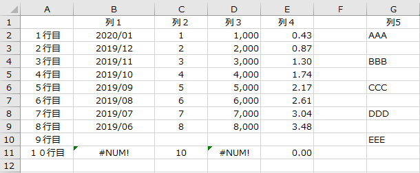
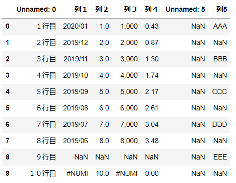
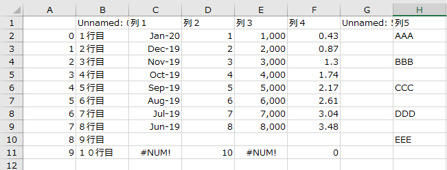
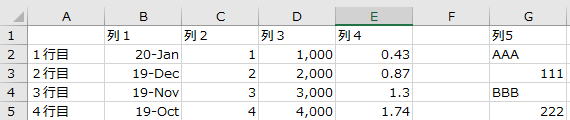

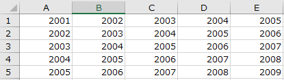

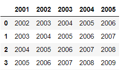
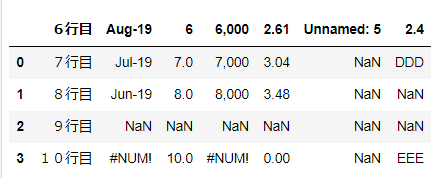
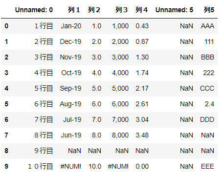
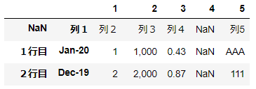

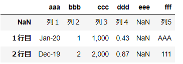
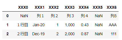
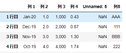


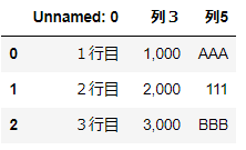
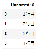
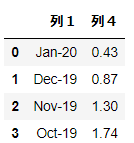
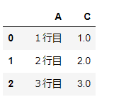
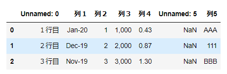
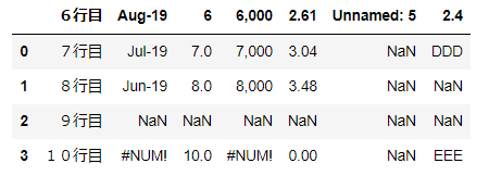
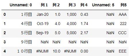
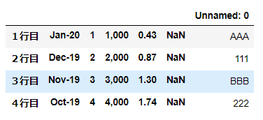
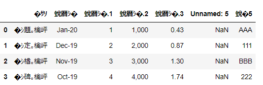
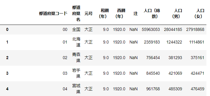
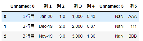
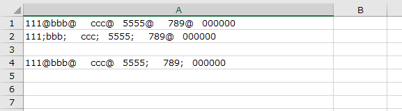
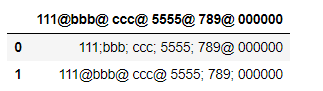
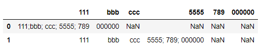
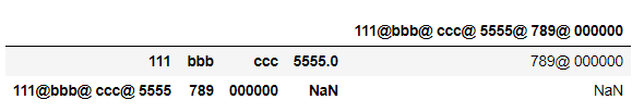
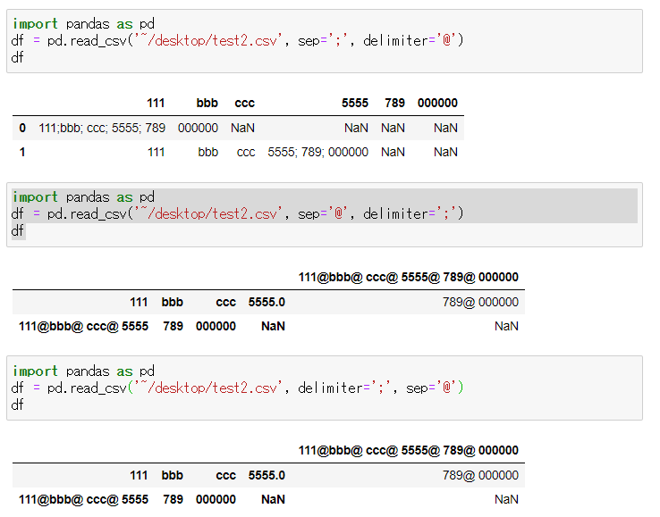
- 投稿日:2020-03-27T16:59:12+09:00
x-meansの使い方
k-means系まとめ
- k-means:クラスターの重心からの二乗誤差を最小化.
- k-medoids:クラスターのmedoid(クラスターに属する点で,非類似度の総和が最小となる点)からの非類似度の総和が最小となるようにEMの手続きを行う.
- x-means:BICに基づいてクラスタの分割を制御.
- g-menas:データが正規分布に基づくと仮定して,アンダーソン・ダリング検定によってクラスタの分割を制御.
- gx-means:上二つの拡張.
- etc(pyclusteringのreadme参照.色々ある)
クラスター数の判定
データを人間が目で見てすぐにクラスター数がわかるならいいのですが,そんなのは稀なので,定量的な判定方法が欲しいところ.
sklearnのチートシートによれば,
- MeanShift
- VBGMM
が推奨されている.
も有用ですが,綺麗にエルボー(グラフがガクッとなる点)が出ることが経験上少なく,クラスター数に迷うことが多かったです.
全自動でクラスター数とクラスタリングをしてくれる方法として,x-meansがあります.
以下,x-meansを含む様々なクラスタリング手法を収録しているライブラリ「pyclustering」の使い方.
pyclusteringの使い方
pyclusteringは,クラスタリングアルゴリズムを集めたライブラリで,pythonとC++の両方で実装されています.
インストール
依存するパッケージ:scipy, matplotlib, numpy, PIL
pip install pyclusteringx-means使用例
x-meansは,k-meansにおけるEMステップに加えて,新たなステップ:あるクラスターが正規分布2つで表されるのと1つで表されるのとどちらが適切か,を判定し,2つが適切な場合はクラスターを2つに分ける,という操作がなされます.
以下,jupyter notebook使用.
import numpy as np
import pandas as pd
import matplotlib.pyplot as plt
from sklearn import cluster, preprocessing

# Wineのデータセット
df_wine_all=pd.read_csv('https://archive.ics.uci.edu/ml/machine-learning-databases/wine/wine.data', header=None)
#品種(0列、1~3)と色(10列)とプロリンの量(13列)を使用する
df_wine=df_wine_all[[0,10,13]]
df_wine.columns = [u'class', u'color', u'proline']

# データの整形
X=df_wine[["color","proline"]]
sc=preprocessing.StandardScaler()
sc.fit(X)
X_norm=sc.transform(X)

# プロット
%matplotlib inline

x=X_norm[:,0]
y=X_norm[:,1]
z=df_wine["class"]
plt.figure(figsize=(10,10))
plt.subplot(4, 1, 1)
plt.scatter(x,y, c=z)
plt.show

# x-means
from pyclustering.cluster.xmeans import xmeans
from pyclustering.cluster.center_initializer import kmeans_plusplus_initializer
xm_c = kmeans_plusplus_initializer(X_norm, 2).initialize()
xm_i = xmeans(data=X_norm, initial_centers=xm_c, kmax=20, ccore=True)
xm_i.process()

# 結果をプロット
z_xm = np.ones(X_norm.shape[0])
for k in range(len(xm_i._xmeans__clusters)):
    z_xm[xm_i._xmeans__clusters[k]] = k+1

plt.subplot(4, 1, 2)
plt.scatter(x,y, c=z_xm)
centers = np.array(xm_i._xmeans__centers)
plt.scatter(centers[:,0],centers[:,1],s=250, marker='*',c='red')
plt.show
上が元々のデータのクラスごとに色付けした図,下がx-meansによるクラスタリング結果.
★印は各クラスの重心です.コード内の
xm_c = kmeans_plusplus_initializer(X_norm, 2).initialize()で,クラスター数の初期値を2に設定していますが,きちんと3つにクラスタリングしてくれています.
xm_i.process()でx-meansを実行しています.x-meansインスタンス(上のコードでは
xm_i)について,学習前と学習後でインスタンス変数を色々見ると,学習結果がどんな感じかがわかると思います.例えばxm_i.__dict__.keys()または
vars(xm_i).keys()で取得できる
dict_keys(['_xmeans__pointer_data', '_xmeans__clusters', '_xmeans__centers', '_xmeans__kmax', '_xmeans__tolerance', '_xmeans__criterion', '_xmeans__ccore'])などを色々見るとよいかと思います.
_xmeans_pointerdata
クラスタリング対象となったデータのコピー.
_xmeans__clusters
各クラスターには,元データ(_xmeans__pointer_data)の何行目が属しているかを表したリスト.
リストの要素数はクラスター数と同じであり,各要素はまたリストになっており,クラスターに属する行の番号が格納されている.
_xmeans__centers
各クラスターのセントロイドの座標(リスト)からなるリスト
_xmeans__kmax
クラスター数の最大値(設定値)
_xmeans__tolerance
x-meansのiterationの停止条件を定める定数です.クラスターの重心の変化の最大値がこの定数を下回ったとき,アルゴリズムが終了します.
_xmeans__criterion
クラスターの分割の判定条件です.デフォルト:BIC
_xmeans__ccore
pythonコードの代わりにC++コードを使うかどうかの設定値です.
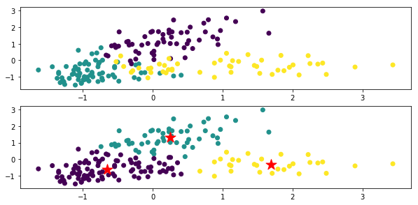
- 投稿日:2020-03-27T16:30:04+09:00
多倍長評価でnumpy.ndarrayを使う
前置き
python3系では標準で整数は無限桁扱うことができ,mpmathパッケージを利用すれば実数(複素数)の多倍長数値演算が可能である.個人的に,numpy.arrayと組み合わせて利用しているのだが,いくつか注意が必要なので個人的な備忘録として注意すべき点を記録する.
多倍長評価のdemo
>>> import python
>>> math.factorial(100)
93326215443944152681699238856266700490715968264381621468592963895217599993229915608941463976156518286253697920827223758251185210916864000000000000000000000000
>>> import mpmath
>>> mpmath.mp.dps = 100
>>> print(mpmath.pi)
3.141592653589793238462643383279502884197169399375105820974944592307816406286208998628034825342117068
精度の確認
python 標準のfloatに関する精度は次のコマンドで確認可能
>>> import sys >>> sys.float_info sys.float_info(max=1.7976931348623157e+308, max_exp=1024, max_10_exp=308, min=2.2250738585072014e-308, min_exp=-1021, min_10_exp=-307, dig=15, mant_dig=53, epsilon=2.220446049250313e-16, radix=2, rounds=1)epsilonは計算機イプシロンで1の次に大きい最小の数とのこと.numpyのarray(ndarray)はC言語で実装されていると何かで読んだので,C言語の型の制約を受ける.実際numpy.arrayを作る際にdtypeが指定される.
numpyの場合finfo(浮動小数点), iinfo(整数)で確認することができnumpy:overflow-error
>>> import numpy as np
>>> np.finfo(np.float)
finfo(resolution=1e-15, min=-1.7976931348623157e+308, max=1.7976931348623157e+308, dtype=float64)
>>> np.finfo(np.float128)
finfo(resolution=1e-18, min=-1.189731495357231765e+4932, max=1.189731495357231765e+4932, dtype=float128)
>>> np.iinfo(np.int)
iinfo(min=-9223372036854775808, max=9223372036854775807, dtype=int64)
から確認できる.float128はCで言うlong doubleであってfloat128(4倍浮動小数点)ではない.Overflowの挙動は
>>> np.array([np.finfo(np.float).max], dtype=np.float) * 2
array([inf])
>>> np.array([np.iinfo(np.int).max], dtype=np.int) + 1
array([-9223372036854775808])
となる.pythonも浮動小数点は倍精度の壁があるので,floatに関してoverflowするのは仕方ないとおもう.しかし,python3はintを無限精度で扱えるのでうっかりoverflowや意図せぬ精度不足に陥ることがある.numpy.arrayでnp.intの精度限界を超えた整数を扱いたければ,dtypeを無指定にするか,dtypeにobjectを指定すれば良い.
つまり
import math
>>> np.array([math.factorial(25)], dtype=np.int)
Traceback (most recent call last):
  File "<ipython-input-46-0451d8765c1b>", line 1, in <module>
    np.array([math.factorial(25)], dtype=np.int)
OverflowError: Python int too large to convert to C long
だが
>>> np.array([math.factorial(25)])
array([15511210043330985984000000], dtype=object)
となる.dtypeをobjectに指定(無指定)するとmpmathのような多倍長浮動小数点も扱える.
多倍長浮動小数(mpmath)でnumpy.arrayをつかう
intの場合と同じ様にdtypeを無指定(or dtype=object)にすれば良い.
>>> import mpmath
>>> mpmath.mp.dps = 50
>>> np.array([mpmath.mpf("1")])/3
array([mpf('0.33333333333333333333333333333333333333333333333333311')], dtype=object)
昔は演算の順序を変えると未定義だと怒られることがあったが,今はdtypeがobjectなのかnp.floatやnp.intなのか意識せずほぼ同等四則演算等の操作が可能(arrayの要素が四則演算可能なら).当然であるが,dtypeがnp.float(やnp.int)のarrayと演算を施すと精度が失われる.
>>> np.array(mpmath.linspace(0, 1, 10)) + np.linspace(0, 10, 10)
array([mpf('0.0'),
       mpf('1.2222222222222222715654677611180684632725185818142358'),
       mpf('2.4444444444444445431309355222361369265450371636284716'),
       mpf('3.6666666666666668146964032833542053898175557454427101'),
       mpf('4.8888888888888890862618710444722738530900743272569433'),
       mpf('6.1111111111111109137381289555277261469099256727430567'),
       mpf('7.3333333333333336293928065667084107796351114908854202'),
       mpf('8.555555555555556345047484177889095412360297309027773'),
       mpf('9.7777777777777781725237420889445477061801486545138865'),
       mpf('11.0')], dtype=object)
計算速度の比較
numpy.arrayで dtype=np.intやnp.floatは計算速度のbest perfomanceがでるだろう.dtype=objectにするとどの程度遅くなるのか確認しておく.
import numpy as np
import mpmath
import time

def addsub(x, imax):
    x0 = np.copy(x)
    time0 = time.time()
    for n in range(imax):
        xx = x + x
        x = xx - x
    print(time.time()-time0, "[sec]", sum(x-x0), x.dtype)

def powpow(x, imax):
    x0 = np.copy(x)
    time0 = time.time()
    for n in range(imax):
        xx = x**(3)
        x = xx**(1/3)
    print(time.time()-time0, "[sec]", float(sum(x-x0)), x.dtype)

imax = 10000
sample = 10000

x = np.arange(0, sample, 1, dtype=np.int)
addsub(x, imax)

x = np.arange(0, sample, 1, dtype=object)
addsub(x, imax)


x = np.arange(0, sample, 1, dtype=np.float)
powpow(x, imax)

x = np.arange(0, sample, 1, dtype=object)
powpow(x, imax)
次が実行結果
0.06765484809875488 [sec] 0 int64

3.387320041656494 [sec] 0 object

8.931994915008545 [sec] -0.00024138918300131706 float64

16.408015489578247 [sec] -0.00024138918300131706 object
arrayの要素がintの場合は,objectに指定すると圧倒的に遅くなる傾向にあるが,一方でfloatに関しては2倍程度と許容の範囲だろう.さてmpmathの場合を考えよう.mpmathはデフォルトの仮数部は15桁なので,15桁と仮数部100桁の場合で計算速度を比較しよう.ただ,上の設定だと数時間ほど掛かりそうなのでimaxを2桁落とす.そのため,上の結果と比較するには計算時間を100倍すれば,おおよそ比較可能.
imax = 100

mpmath.mp.dps=100
x = np.array(mpmath.arange(0, sample, 1), dtype=object)
powpow(x, imax)
次が実行結果
15.098075151443481 [sec] -2.4139151442170714e-06 objectmpmath,仮数部15桁で計算量を1/100にしているのでだいたい100倍程度かかる.
ちなみにpowpowの定義では精度は改善されない.なぜなら$x^{1/3}$とした際に指数部がpythonのfloatで評価されてしまうため15桁以降は意味の無い数字となる.そこでpowpowを少し修正して
def papawpowpow(x, imax):
    x0 = np.copy(x)
    time0 = time.time()
    for n in range(imax):
        xx = x**(3)
        x = xx**(mpmath.mpf("1/3"))
    print(time.time()-time0, "[sec]", float(sum(x-x0)), x.dtype)
として実行すると
21.777454376220703 [sec] 1.5530282978129947e-91 objectmpmath.mp.dps=100 x = np.array(mpmath.arange(0, sample, 1), dtype=object) papawpowpow(x, imax)ちなみにarrayを使わずにelementwiseで評価すると
def elewisepapawpowpow(x, imax):
    x0 = x[:]
    time0 = time.time()
    for n in range(imax):
        xx = [x1**(3) for x1 in x]
        x =  [x1**(mpmath.mpf("1/3")) for x1 in xx]
    diff = [x[i] - x0[i] for i in range(len(x0))]
    print(time.time()-time0, "[sec]", float(sum(diff)), type(x))
となる.
28.9152569770813 [sec] 1.5530282978129947e-91 <class 'list'>計算速度はnumpy.arrayの場合と比較して30%弱早く,コーディングも使い慣れたnumpy.arrayを使った方がスッキリする.
実行環境
$ lscpu
アーキテクチャ:                      x86_64
CPU 操作モード:                      32-bit, 64-bit
バイト順序:                          Little Endian
CPU:                                 4
オンラインになっている CPU のリスト: 0-3
コアあたりのスレッド数:              1
ソケットあたりのコア数:              4
ソケット数:                          1
NUMA ノード数:                       1
ベンダー ID:                         AuthenticAMD
CPU ファミリー:                      23
モデル:                              17
モデル名:                            AMD Ryzen 3 2200G with Radeon Vega Graphics
ステッピング:                        0
CPU MHz:                             1479.915
CPU 最大 MHz:                        3500.0000
CPU 最小 MHz:                        1600.0000
BogoMIPS:                            7000.24
仮想化:                              AMD-V
L1d キャッシュ:                      32K
L1i キャッシュ:                      64K
L2 キャッシュ:                       512K
L3 キャッシュ:                       4096K
NUMA ノード 0 CPU:                   0-3
フラグ:                              fpu vme de pse tsc msr pae mce cx8 apic sep mtrr pge mca cmov pat pse36 clflush mmx fxsr sse sse2 ht syscall nx mmxext fxsr_opt pdpe1gb rdtscp lm constant_tsc rep_good nopl nonstop_tsc cpuid extd_apicid aperfmperf pni pclmulqdq monitor ssse3 fma cx16 sse4_1 sse4_2 movbe popcnt aes xsave avx f16c rdrand lahf_lm cmp_legacy svm extapic cr8_legacy abm sse4a misalignsse 3dnowprefetch osvw skinit wdt tce topoext perfctr_core perfctr_nb bpext perfctr_llc mwaitx cpb hw_pstate sme ssbd sev ibpb vmmcall fsgsbase bmi1 avx2 smep bmi2 rdseed adx smap clflushopt sha_ni xsaveopt xsavec xgetbv1 xsaves clzero irperf xsaveerptr arat npt lbrv svm_lock nrip_save tsc_scale vmcb_clean flushbyasid decodeassists pausefilter pfthreshold avic v_vmsave_vmload vgif overflow_recov succor smca
$ cat /proc/cpuinfo | grep MHz cpu MHz : 1624.805 cpu MHz : 1500.378 cpu MHz : 3700.129 cpu MHz : 2006.406
- 投稿日:2020-03-27T16:11:25+09:00
PythonでExcel文字列の一部に色をつけたい
はじめに
タイトルの通りですが、Pythonを使用してExcelファイルを読み込み、セル内に書き込まれている文字列の一部に色をつけて出力します。
当初はopenpyxlで行おうと思っていましたが、どうも目的の動きはできなそうだったのでxlsxwriterのwrite_rich_stringを使用して実現することにしました。
ですが、xlsxwriterは読み込みができないので、読み込み部分はopenpyxl、書き込み部分はxlsxwriterで行おうと思います。
Pythonを選んだのは、自分があまり触ったことがないからです。やること
1.PythonでExcelを読み込み
openpyxlimport openpyxl # openpyxlでファイルを開く iptbook = openpyxl.load_workbook(filename='test.xlsx') # シート選択 iptsheet = iptbook.worksheets[0] # セルの文字列を取得 cellvalue = iptsheet.cell(row=1, column=1).value # 終了 iptbook.close()2.セル内の文字列の一部に色をつけて出力
xlsxwriterimport xlsxwriter # xlsxwriterでブックを作成 optbook = xlsxwriter.Workbook('opt.xlsx') # xlsxwriterでシートを追加 optsheet = optbook.add_worksheet() # 書式を定義 red = optbook.add_format({'color': 'red'}) # 文字を分割 splitvalue = cellvalue.split() # リッチテキストで書き込み optsheet.write_rich_string('A1', red, splitvalue[0], splitvalue[1]) # 終了 optbook.close()結果
実行前と後のファイルになります。
参考にさせていただいた記事
Example: Writing “Rich” strings with multiple formats
Excelで1セル内に複数の書式(フォント)が混在するようなものをPythonで扱いたい
おわりに
リッチテキストであれば、色に限らず線の太さやフォントも変えることができます。
今回は2つのライブラリを組み合わせて使用することで実現ができました。
よりよい方法をご存じの方がいましたら教えてくださると嬉しいです。


- 投稿日:2020-03-27T16:03:29+09:00
Cython, Numbaを簡単に動かしてみる
概略
numbaとは,JIT(just-in-time)コンパイラを使ってPythonを動作させるモジュール,
Cythonとは,Pythonみたいに書けるけどC/C++と同様に事前コンパイルするプログラミング言語です.とりあえず動かしてみる
以下,Jupyter Notebook上での処理になります.
Anaconda, python 3.7.3 を使用.
フィボナッチ数列のn番目を生成するコードで,python, numba, cython, 型指定つきcython, の4つで速度比較をしてみます.
まずは普通のpython
def python_fib(n):
    a, b = 0., 1.
    for i in range(n):
        a, b = a + b, a
    return a
timeitモジュールで,フィボナッチ数列の1000番目の数を計算する処理にかかる時間を計測してみます.%timeit python_fib(1000)10000 loops, best of 3: 33.6 µs per loop平均して 33.6マイクロ秒かかったようです.
この場合、コマンド %timeit は以下の処理を行っています.
- python_fib(1000)を10000回実行し、総実行時間を保存.
- python_fib(1000)を10000回実行し、総実行時間を保存.
- python_fib(1000)を10000回実行し、総実行時間を保存.
- 3回実行した中で最も短い実行時間を取得し、それを10000で割った値を、10000の最短実行時間として出力。
ループ回数(ここでは10000ループ)は、
%timeitの機能によって自動調整されており,測定するコードの実行速度に応じて変化します.Numbaでコンパイルした場合
numbaは
pipでインストールできます.pip install numbanumbaの使い方は非常に簡単で,
@jitデコレータをつけるだけです.from numba import jit @jit def numba_fib(n): a, b = 0.0, 1.0 for i in range(n): a, b = a + b, a return a処理時間を計測します.
%timeit numba_fib(1000)The slowest run took 77684.24 times longer than the fastest. This could mean that an intermediate result is being cached. 1000000 loops, best of 3: 1.26 µs per loop1.26マイクロ秒!26倍もの高速化になりました.
Cython を使用した場合
jupyterでは,以下のマジックコマンドでcythonがロードできます.
%load_ext Cython%%cython を最初に入れることで,コンパイルと最適化が行われます.
%%cython def cython_fib(n): a, b = 0.0, 1.0 for i in range(n): a, b = a + b, a return a%timeit cython_fib(1000)100000 loops, best of 3: 8.22 µs per loop8.22マイクロ秒.何もしなくても4倍程度には速くなりましたね.
最後に,型指定をした後に,cythonでコンパイルした場合.
%%cython def cython_fib2(int n): a, b = 0., 1. for i in range(n): a, b = a + b, a return a%timeit cython_fib2(1000)The slowest run took 7.27 times longer than the fastest. This could mean that an intermediate result is being cached. 1000000 loops, best of 3: 984 ns per loop0.984マイクロ秒!34倍も早くなりました.
最後に
上のような簡単な処理なら,numbaやcythonで動かすことは容易ですが,複雑な処理になると対応できないケースがでてきます.
速度を求める場合には早めに別言語に切り替えたり,マルチプロセスやハードウェア選定から検討したほうがいいかもしれません.
- 投稿日:2020-03-27T15:36:12+09:00
AtCoder Beginner Contest 083 過去問復習
所要時間
感想
うーーん。FXが気になってしょうがない。相場気になりすぎて勉強が手につかないのやばいですね…。
解決方法が思いつきませんが、精神力が流石に足りない。A問題
足し算したやつを比較すれば良いです。
三項演算子を使いました。answerA.pya,b,c,d=map(int,input().split()) print("Left" if (a+b)>(c+d) else "Right" if (a+b)<(c+d) else "Balanced")B問題
1からnまで順に数え上げれば良いです。
answerB.pyn,a,b=map(int,input().split()) ans=0 for i in range(1,n+1): s=0 j=i while j!=0: s+=(j%10) j//=10 if a<=s<=b:ans+=i print(ans)C問題
kをそのまま使用したところおそらく計算誤差で1ケースだけ落ちました。logの計算など整数でない計算は誤差に注意するということを当たり前ではありますが忘れないようにしたいです。
また、二つ目のコードはO(log(x/y))で通せることを意識して丁寧に書いたコードになります。answerC.pyimport math x,y=map(int,input().split()) k=math.floor(math.log2(y/x)) for i in range(k+3): if x*(2**i)>y: print(i) breakanswerC_better.pyimport math x,y=map(int,input().split()) ans=0 while x<=y: x*=2 ans+=1 print(ans)D問題
初めはサンプル例だけみて適当に0と1の多い方としていましたが、そこまで簡単ではありませんでした。
このような反転をする問題ではその反転の操作で選択した部分と選択してない部分で関係性が逆になることがわかります。つまり、[l,r]を反転させた場合は文字列の長さをnとし1-indexで考えた時、[1,l-1],[r+1,n]の二つの部分と[l,r]の部分の関係性が変わります。
したがって、0と1が入れ替わってる場所については隣同士を同じにしなければならないです。ここで、入れ替わってる場所がk,k+1の場合、その二つを同じにするために[v,k],[k+1,w]を選択して反転させる必要があります。ここで、題意より選択する部分できるだけ長くしたく、その長さは自明にv=1の時もしくはw=nの時です。したがって、入れ替わってる場所についてmax([1,k]の長さ,[k+1,n]の長さ)を求めていきその中で最短のものが答えになります。
また、全て同じ場合は答えはnになることにも注意が必要です。(ansに適当にinfを設定していたので痛い目をみました。)answerD.pys=input() l=len(s) ans=l for i in range(l-1): if s[i]!=s[i+1]: ne=max(i+1,l-i-1) ans=min(ans,ne) print(ans)
- 投稿日:2020-03-27T15:22:47+09:00
画像処理 | predicting species from images
この記事は前回の記事の続き。今回はmachine learningを使って、modelをtrainして、画像のcategoryを分類するものだ。これもdata campから学んだ物だから、興味あるかたはdata campをチェックしてください。ここからは英語にします。
Import Python Libraries
This time we are going to use scikit learn and PIL to handle the image processing and machine learning.
# used to change filepaths
import os

import matplotlib as mpl
import matplotlib.pyplot as plt
from IPython.display import display
%matplotlib inline

import pandas as pd
import numpy as np

from PIL import Image

from skimage.feature import hog
from skimage.color import rgb2grey

from sklearn.preprocessing import StandardScaler
from sklearn.decomposition import PCA

# import train_test_split from sklearn's model selection module
from sklearn.model_selection import train_test_split

# import SVC from sklearn's svm module
from sklearn.svm import SVC

# import accuracy_score from sklearn's metrics module
from sklearn.metrics import roc_curve, auc, accuracy_score
Display image of each bee type
Now that we have all of our imports ready, it is time to look at some images. We will load our labels.csv file into a dataframe called labels, where the index is the image name (e.g. an index of 1036 refers to an image named 1036.jpg) and the genus column tells us the bee type. genus takes the value of either 0.0 (Apis or honey bee) or 1.0 (Bombus or bumble bee).
The function get_image converts an index value from the dataframe into a file path where the image is located, opens the image using the Image object in Pillow, and then returns the image as a numpy array.
We'll use this function to load the sixth Apis image and then the sixth Bombus image in the dataframe.
# load the labels using pandas
labels = pd.read_csv("datasets/labels.csv", index_col=0)

# show the first five rows of the dataframe using head
display(labels.head())

def get_image(row_id, root="datasets/"):
    """
    Converts an image number into the file path where the image is located,
    opens the image, and returns the image as a numpy array.
    """
    filename = "{}.jpg".format(row_id)
    file_path = os.path.join(root, filename)
    img = Image.open(file_path)
    return np.array(img)

# subset the dataframe to just Apis (genus is 0.0) get the value of the sixth item in the index
apis_row = labels[labels.genus == 0.0].index[5]

# show the corresponding image of an Apis
plt.imshow(get_image(apis_row))
plt.show()

# subset the dataframe to just Bombus (genus is 1.0) get the value of the sixth item in the index
bombus_row = labels[labels.genus == 1.0].index[5]

# show the corresponding image of a Bombus
plt.imshow(get_image(bombus_row))
plt.show()
Image manipulation with rgb2grey
scikit-image has a number of image processing functions built into the library, for example, converting an image to greyscale. The rgb2grey function computes the luminance of an RGB image using the following formula Y = 0.2125 R + 0.7154 G + 0.0721 B.
Image data is represented as a matrix, where the depth is the number of channels. An RGB image has three channels (red, green, and blue) whereas the returned greyscale image has only one channel. Accordingly, the original color image has the dimensions 100x100x3 but after calling rgb2grey, the resulting greyscale image has only one channel, making the dimensions 100x100x1.
# load a bombus image using our get_image function and bombus_row from the previous cell
bombus = get_image(bombus_row)

# print the shape of the bombus image
print('Color bombus image has shape: ', ...)

# convert the bombus image to greyscale
grey_bombus = rgb2grey(bombus)

# show the greyscale image
plt.imshow(grey_bombus, cmap=mpl.cm.gray)

# greyscale bombus image only has one channel
print('Greyscale bombus image has shape: ', 1)
Histogram of oriented gradients
Now we need to turn these images into something that a machine learning algorithm can understand. Traditional computer vision techniques have relied on mathematical transforms to turn images into useful features. For example, you may want to detect edges of objects in an image, increase the contrast, or filter out particular colors.
We've got a matrix of pixel values, but those don't contain enough interesting information on their own for most algorithms. We need to help the algorithms along by picking out some of the salient features for them using the histogram of oriented gradients (HOG) descriptor. The idea behind HOG is that an object's shape within an image can be inferred by its edges, and a way to identify edges is by looking at the direction of intensity gradients (i.e. changes in luminescence).
HOG
An image is divided in a grid fashion into cells, and for the pixels within each cell, a histogram of gradient directions is compiled. To improve invariance to highlights and shadows in an image, cells are block normalized, meaning an intensity value is calculated for a larger region of an image called a block and used to contrast normalize all cell-level histograms within each block. The HOG feature vector for the image is the concatenation of these cell-level histograms.
# run HOG using our greyscale bombus image
hog_features, hog_image = hog(grey_bombus,
                              visualize=True,
                              block_norm='L2-Hys',
                              pixels_per_cell=(16, 16))

# show our hog_image with a grey colormap
plt.imshow(hog_image, cmap=mpl.cm.gray)
Create image features and flatten into a single row
Algorithms require data to be in a format where rows correspond to images and columns correspond to features. This means that all the information for a given image needs to be contained in a single row.
We want to provide our model with the raw pixel values from our images as well as the HOG features we just calculated. To do this, we will write a function called create_features that combines these two sets of features by flattening the three-dimensional array into a one-dimensional (flat) array.
def create_features(img):
    # flatten three channel color image
    color_features = img.flatten()
    # convert image to greyscale
    grey_image = rgb2grey(img)
    # get HOG features from greyscale image
    hog_features = hog(grey_image, block_norm='L2-Hys', pixels_per_cell=(16, 16))
    # combine color and hog features into a single array
    flat_features = np.hstack([color_features, hog_features])
    return flat_features

bombus_features = create_features(bombus)

# print shape of bombus_features
print(bombus_features.shape)
Loop over images to preprocess
Above we generated a flattened features array for the bombus image. Now it's time to loop over all of our images. We will create features for each image and then stack the flattened features arrays into a big matrix we can pass into our model.
In the create_feature_matrix function, we'll do the following:
- Load an image
- Generate a row of features using the create_features function above
- Stack the rows into a features matrix
In the resulting features matrix, rows correspond to images and columns to features.
def create_feature_matrix(label_dataframe):
    features_list = []

    for img_id in label_dataframe.index:
        # load image
        img = get_image(img_id)
        # get features for image
        image_features = create_features(img)
        features_list.append(image_features)

    # convert list of arrays into a matrix
    feature_matrix = np.array(features_list)
    return feature_matrix

# run create_feature_matrix on our dataframe of images
feature_matrix = create_feature_matrix(labels)
Scale feature matrix + PCA
Our features aren't quite done yet. Many machine learning methods are built to work best with data that has a mean of 0 and unit variance. Luckily, scikit-learn provides a simple way to rescale your data to work well using StandardScaler. They've got a more thorough explanation of why that is in the linked docs.
Remember also that we have over 31,000 features for each image and only 500 images total. To use an SVM, our model of choice, we also need to reduce the number of features we have using principal component analysis (PCA).
PCA is a way of linearly transforming the data such that most of the information in the data is contained within a smaller number of features called components. Below is a visual example from an image dataset containing handwritten numbers. The image on the left is the original image with 784 components. We can see that the image on the right (post PCA) captures the shape of the number quite effectively even with only 59 components.
Our features aren't quite done yet. Many machine learning methods are built to work best with data that has a mean of 0 and unit variance. Luckily, scikit-learn provides a simple way to rescale your data to work well using StandardScaler. They've got a more thorough explanation of why that is in the linked docs.
Remember also that we have over 31,000 features for each image and only 500 images total. To use an SVM, our model of choice, we also need to reduce the number of features we have using principal component analysis (PCA).
In our case, we will keep 500 components. This means our feature matrix will only have 500 columns rather than the original 31,296.
# get shape of feature matrix
print('Feature matrix shape is: ', feature_matrix.shape)

# define standard scaler
ss = StandardScaler()
# run this on our feature matrix
bees_stand = ss.fit_transform(feature_matrix)

pca = PCA(n_components=500)
# use fit_transform to run PCA on our standardized matrix
bees_pca = pca.fit_transform(bees_stand)
# look at new shape
print('PCA matrix shape is: ', bees_pca.shape)
Split into train and test sets
Now we need to convert our data into train and test sets. We'll use 70% of images as our training data and test our model on the remaining 30%. Scikit-learn's train_test_split function makes this easy.
X_train, X_test, y_train, y_test = train_test_split(bees_pca,
                                                    labels.genus.values,
                                                    test_size=.3,
                                                    random_state=1234123)

# look at the distrubution of labels in the train set
pd.Series(y_train).value_counts([0.0,1.0])
Train model
It's finally time to build our model! We'll use a support vector machine (SVM), a type of supervised machine learning model used for regression, classification, and outlier detection." An SVM model is a representation of the examples as points in space, mapped so that the examples of the separate categories are divided by a clear gap that is as wide as possible. New examples are then mapped into that same space and predicted to belong to a category based on which side of the gap they fall."
Here's a visualization of the maximum margin separating two classes using an SVM classifier with a linear kernel.SVM
Since we have a classification task -- honey or bumble bee -- we will use the support vector classifier (SVC), a type of SVM. We imported this class at the top of the notebook.
SVM
# define support vector classifier
svm = SVC(kernel='linear', probability=True, random_state=42)

# fit model
svm.fit(X_train, y_train)
Score Model
Now we'll use our trained model to generate predictions for our test data. To see how well our model did, we'll calculate the accuracy by comparing our predicted labels for the test set with the true labels in the test set. Accuracy is the number of correct predictions divided by the total number of predictions. Scikit-learn's accuracy_score function will do math for us. Sometimes accuracy can be misleading, but since we have an equal number of honey and bumble bees, it is a useful metric for this problem.
# generate predictions
y_pred = svm.predict(X_test)

# calculate accuracy
accuracy = accuracy_score(y_test, y_pred)
print('Model accuracy is: ', accuracy)
ROC curve + AUC
Above, we used svm.predict to predict either 0.0 or 1.0 for each image in X_test. Now, we'll use svm.predict_proba to get the probability that each class is the true label. For example, predict_proba returns [0.46195176, 0.53804824] for the first image, meaning there is a 46% chance the bee in the image is an Apis (0.0) and a 53% chance the bee in the image is a Bombus (1.0). Note that the two probabilities for each image always sum to 1.
Using the default settings, probabilities of 0.5 or above are assigned a class label of 1.0 and those below are assigned a 0.0. However, this threshold can be adjusted. The receiver operating characteristic curve (ROC curve) plots the false positive rate and true positive rate at different thresholds. ROC curves are judged visually by how close they are to the upper lefthand corner.
The area under the curve (AUC) is also calculated, where 1 means every predicted label was correct. Generally, the worst score for AUC is 0.5, which is the performance of a model that randomly guesses. See the scikit-learn documentation for more resources and examples on ROC curves and AUC.
# predict probabilities for X_test using predict_proba
probabilities = svm.predict_proba(X_test)

# select the probabilities for label 1.0
y_proba = probabilities[:,1]

# calculate false positive rate and true positive rate at different thresholds
false_positive_rate, true_positive_rate, thresholds = roc_curve(y_test, y_proba, pos_label=1)

# calculate AUC
roc_auc = auc(false_positive_rate, true_positive_rate)

plt.title('Receiver Operating Characteristic')
# plot the false positive rate on the x axis and the true positive rate on the y axis
roc_plot = plt.plot(false_positive_rate,
                    true_positive_rate,
                    label='AUC = {:0.2f}'.format(roc_auc))

plt.legend(loc=0)
plt.plot([0,1], [0,1], ls='--')
plt.ylabel('True Positive Rate')
plt.xlabel('False Positive Rate');
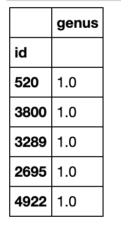
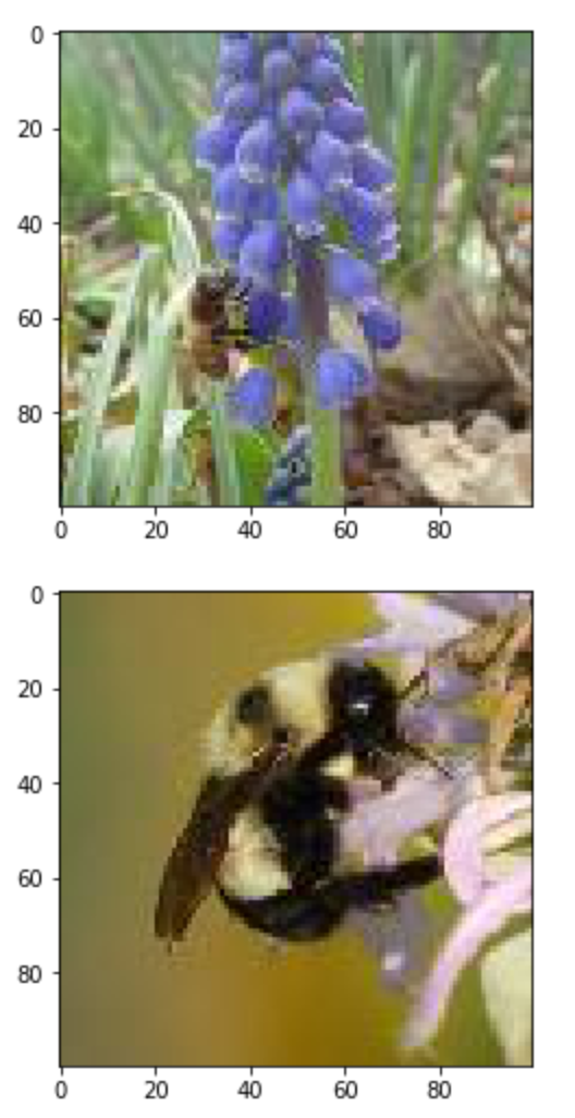
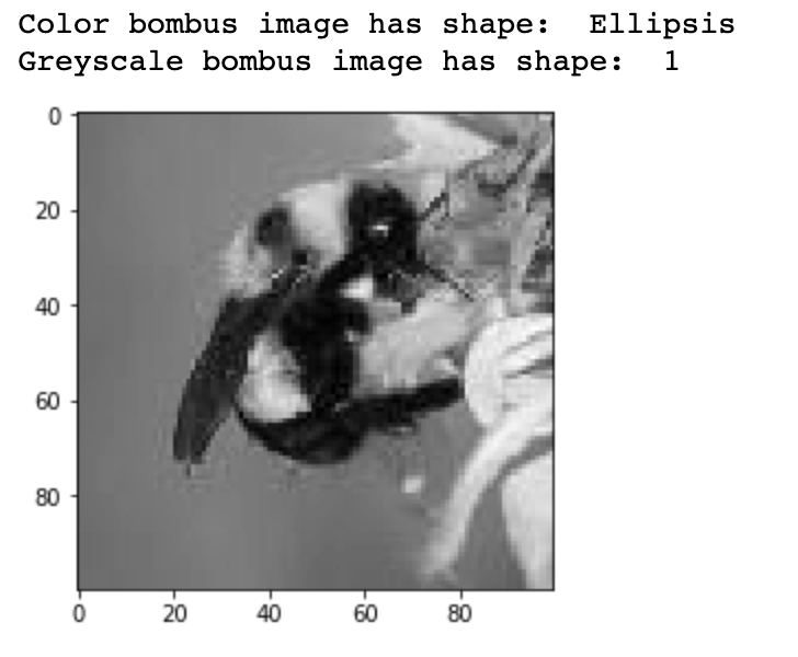
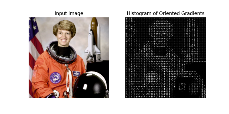
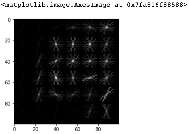
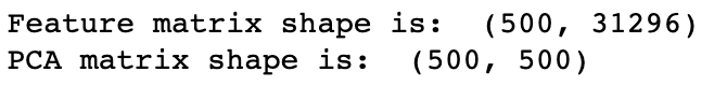
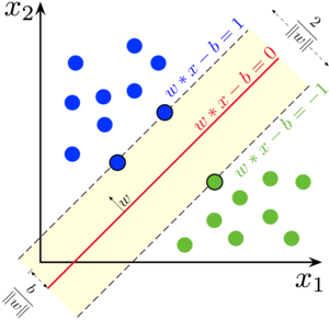

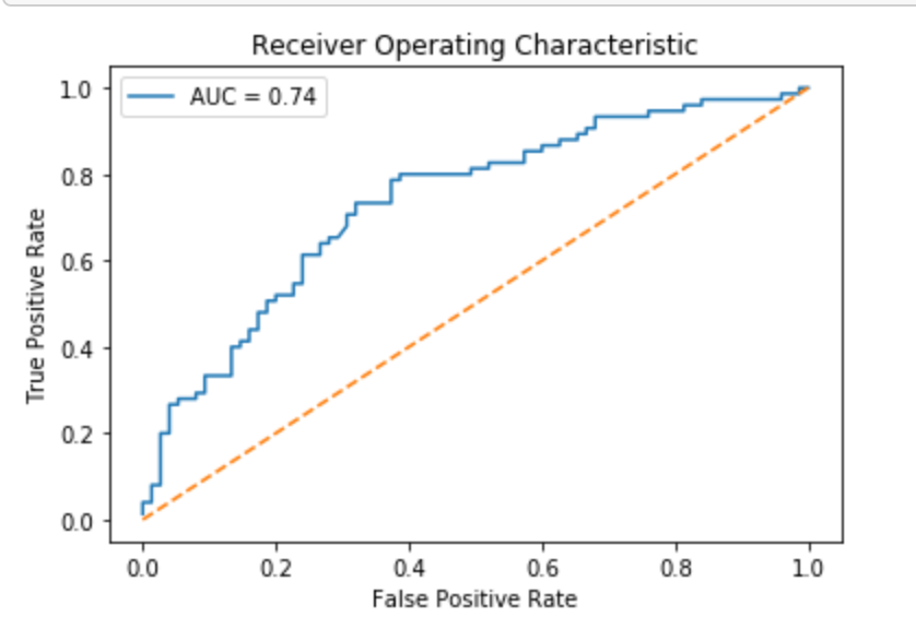
- 投稿日:2020-03-27T14:57:11+09:00
Blender python でシーン編集するメモ(W.I.P.)
対象
- Blender 2.82a or later
API としては Maya mel が python になった感じが強いでしょうか.
パラメータやアトリビュートにアクセスして, 値を取得したり変更したい
たとえばマテリアルで色を変えたいなど.
UI で右クリック -> Copy Data Path して, python console などに貼り付ければ, どのようにアクセスすればいいのかいくらかわかります.
ただ, これはノードを起点としての階層なので, node_tree も取得する必要があります.
node_tree については, 以下のようにしてアクセス.
Blender のノードを Python から操作する
https://dskjal.com/blender/process-node-from-python.html位置などを変えたい
T.B.W.
点群をプロットしたい
Blender + Pythonでポイントクラウドを可視化する
https://ksknw.hatenablog.com/entry/2019/10/29/192026bpy.ops.mesh.primitive_uv_sphere_add(location=(x, y, z))のような感じで sphere を作ることができる.
より効率的に行うなら, particle として表現でしょうか.
形状データへのアクセス
T.B.W.
- 頂点座標
- 法線
- UV データ
- Vertex color
- Skin weight
- Edge, face
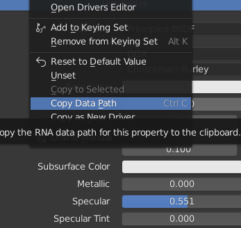
- 投稿日:2020-03-27T14:31:57+09:00
VSCodeでのEV3Micropyhonプログラミングに自動補完の機能を追加する
LEGO Mindstorms EV3は,公式でPython(EV3MicroPython=Pybricks)に対応しており,Microsoft社のフリーの統合開発環境であるVSCode(Visual Studio Code editor)の拡張機能とEV3のファームウェアが公開されています1.
VSCodeに拡張機能を追加するだけで簡単に使えるので,EV3を使ったテキストプログラミングの入門にオススメなのですが,コーディングするにあたって不満点が一つあります.それは,自動補完の機能がないということです.
ここでは,VSCodeでEV3MicropythonのAPIを自動補完するための手順を紹介します.
手順
手順をざっくり説明すると,ワークスペースにpybricksのAPIフォルダをコピーし,VSCodeのAutoComplete Extentionにフォルダパスを追加する,といったものです.(正攻法でないと思うので,より簡単で汎用性のある方法があれば教えてください...)
pybricks-apiのダウンロード
pybricksのAPIフォルダは,GitHubからダウンロードすることができます2.
https://github.com/pybricks/pybricks-api
"Clone of Download"->"Download ZIP"をクリックし,ZIPファイルを展開したら,pybricksフォルダをVSCodeのワークスペース直下にコピーします.VSCodeの自動補完設定
基本設定->設定から,Python > Auto Complete Extra Pathsに設定を追加します(事前にPythonの拡張機能を入れておく必要があるかも).ワークスペース内のsetting.jasonファイルを開き,下記のように追加したいモジュールのパスを書いておきます3.
setting.jason{ "python.autoComplete.extraPaths": [ "./pybricks/" ], }VSCodeを再起動すると,pubricksのAPIが自動補完されるようになります.
(画像は,Motorクラスのインスタンスであるleft_motorを記述した際に,メソッドの候補が表示されている様子)
参考
Pybricks
VSCodeでPythonの自作モジュールにも補完を効かせる方法
VSCodeでなぜか「unresolved import」が出る時の対処法
https://education.lego.com/ja-jp/support/mindstorms-ev3/python-for-ev3 ↩
ここで公開されているのは,ベータ版のVer.2.0のAPIとなります.LEGO Educationで一般公開されているVer.1.0とは少し異なるものの,ほとんどのクラスやメソッド名は共通しているので,大体の自動補完はカバーできます. ↩
ワークスペースにsetting.jasonが存在していない場合は,ワークスペースとして保存されていない可能性があります.「名前をつけてワークスペースを保存」でワークスペースとして保存してください. ↩
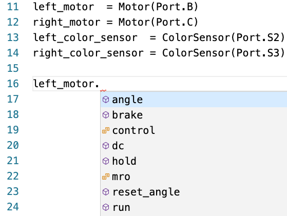
- 投稿日:2020-03-27T13:45:59+09:00
Amazon Comprehendの感情分析をAWS CLIで行ってみた。
Amazon Comprehendの感情分析をAWS CLIで行ってみた。
Amazon Comprehendでできるらしい。
DetectSentimentのところを参照
https://docs.aws.amazon.com/comprehend/latest/dg/API_DetectSentiment.html今回PythonでやってみるのでPython用のを見る。
https://boto3.amazonaws.com/v1/documentation/api/latest/reference/services/comprehend.html#Comprehend.Client.detect_sentiment一番上に何をインポートすればいいか書いてある。
https://boto3.amazonaws.com/v1/documentation/api/latest/reference/services/comprehend.htmlコードはこんな感じ。
import boto3 client = boto3.client('comprehend') response = client.detect_sentiment( Text='東京オリンピックが延期になるなんて、まさにアキラの世界みたいだ。', LanguageCode='ja' ) print(response)結果はこんな感じ。
{'Sentiment': 'NEUTRAL', 'SentimentScore': {'Positive': 0.12571793794631958, 'Negative': 0.006899271160364151, 'Neutral': 0.8673694729804993, 'Mixed': 1.3250895790406503e-05}, 'ResponseMetadata': {'RequestId': 'e458bcfd-c85e-4314-bb01-f11b8e72ec8f', 'HTTPStatusCode': 200, 'HTTPHeaders': {'x-amzn-requestid': 'e458bcfd-c85e-4314-bb01-f11b8e72ec8f', 'content-type': 'application/x-amz-json-1.1', 'content-length': '164', 'date': 'Fri, 27 Mar 2020 04:44:21 GMT'}, 'RetryAttempts': 0}}
- 投稿日:2020-03-27T12:23:30+09:00
amazon linux2上でのPython環境構築方法
メモとして残しておく
# Amazon Linux コンパイラ周りのインストール yum install gcc gcc-c++ make git openssl-devel bzip2-devel zlib-devel readline-devel sqlite-devel xz-devel ## pyenvのインストールとpath通す git clone https://github.com/yyuu/pyenv.git ~/.pyenv echo 'export PYENV_ROOT="$HOME/.pyenv"' >> ~/.bash_profile echo 'export PATH="$PYENV_ROOT/bin:$PATH"' >> ~/.bash_profile echo 'eval "$(pyenv init -)"' >> ~/.bash_profile source ~/.bash_profile ## pythonのインストール pyenv install 3.8.1 pyenv global 3.8.1Pythonのversion確認
$ python Python 3.8.1 (default, Feb 2 2020, 08:37:37) [GCC 8.3.0] on linux Type "help", "copyright", "credits" or "license" for more information. >>>
- 投稿日:2020-03-27T10:27:01+09:00
備忘録:/etc/shadow を直接変更する
Linux NAS 箱などの /etc/shadow に保存されているパスワードがわからくなったときの手段。
- HDD を取り外して Linux (PC) に接続 (mount)
- python3 でハッシュを作る
- mount したパーティションにある /etc/shadow を編集
python3 によるパスワード ハッシュ生成
$ python3 >>> import crypt >>> crypt.crypt('<password>', crypt.mksalt()) '$.$..$...'
- 投稿日:2020-03-27T10:21:06+09:00
AI部・開発チームの働き方(私の場合)
本記事ではAIテクノロジー部の開発チームに所属する、私、小川の働き方を紹介します。
なお、本記事は私の場合の紹介です。
働き方はメンバーごとに異なりますし、家族構成によっても異なります。
私の場合は結婚していますが、子供はいないです。また部が異なる場合も働き方は違います。
本記事ではあくまで、AIテクノロジー部の私(小川雄太郎)の働き方、1週間を紹介します。
なぜ今の会社から転職しないのか
ときおり、「なぜ小川は電通国際情報サービス(ISID)で働いているの?他に転職しないの?」
と聞かれるのですが、現時点、転職していない理由の大きな1つが
「ISIDが非常に働きやすく、仕事とプライベート(自己学習)が両立しやすい環境」
です。
その実態を紹介します。
「基本ルール」
まず会社の基本ルールですが、
- 所定労働時間は7時間
- 所定の標準勤務時間は9:30~17:30(1時間休憩を含む)
です。
多くの企業様は、標準労働時間は8時間(7時間45分)が多いですが、
ISIDは7時間です。8時間と比べると、毎日1時間、労働時間が少ないです。
1時間×20日/月だと、月に20時間少ないことになります。
イメージ的には、
「8時間の企業に比べると、毎月、3日ほど祝日が多い」感じです。
その分、勤務時間外で自分でいろいろ勉強する時間がとれるので、
自己成長しやすく、この労働時間のルールが気に入っています。残業時間は、
openwork(旧vorkers)を見ると、月37時間と記載されていますが、
https://www.vorkers.com/company.php?m_id=a0910000000GVZZ公式な数値では、全社平均で25.5時間/月(2018年度実績)のようです。
(ISID公式 https://www.isid.co.jp/neo-pro/faq/)私の残業時間も基本的には25~30時間程度です。
また、残業時間は月ごとで計算するので、
例えば、
月曜日に9時間働いて(2時間残業)、
火曜日は、前日の残業2時間分、短く働き、5時間勤務して帰ります。
(仕事のスケジュール上可能なら)「フレックス制」
標準労働時間は先に紹介した通り、7時間ですが、フレックス制でコアタイムのみ存在しています。
コアタイムは部によって異なります。私の所属するAIテクノロジー部は9:30-12:00がコアタイムです。
そのため、基本的には皆、9:30に出社して、17:30から18:30あたりで帰ります。入社時に入った部の場合は13:00-15:30がコアタイムだったので、
11時や昼から来る人が多かったです(その分、皆夜遅めまで働いていました)なお私の場合は、周囲から”おじいちゃん”と呼ばれるくらいに朝型です。
基本的には朝7:30から働き、7時間+休憩1時間の8時間勤務で、15:30に退社します。
(15:30に仕事が終わり、帰りに実家に電話をかけると、
親から「あんた、ほんまに仕事行っているの?」と心配されます)「テレワーク」
基本的には週に2日間のテレワークが取得できます。
週3日以上テレワークしたい場合は、上長の許可を得れば可能です。基本的には、私は週2日はテレワーク(在宅)です。
また、負荷が高い週が続いた際には、
次の週は、まるまる1週間を全部在宅勤務にして、身体を休めながら働くこともあります。テレワークの場合、「社内の会議やお客様との打ち合わせはどうするのか?」が問題です。
まず「部の定例会議」が毎週あります。
部の定例会議は、基本的にはテレワークで参加します。
そして部長が自分で会議資料などを皆に画面共有し、会議を進めます。そもそも、関西支社のメンバもいるので、テレカンが基本です。
そのため、テレワークでも問題はありません。社内の会議も同じです。
なお、お客様との打ち合わせなどの場合は、
・ある程度関係性ができている
・移動時間がお互いにとってもったいない
・その場にリアルにいなくても会議のアウトプットの質は落ちないその場合は、基本的にはテレカンで打ち合わせや進捗報告、相談会などを実施します。
ただし、社内の会議でも、お客様との会議でも、
・私がファシリテートする必要がある場合
・非常に重要度が高い場合
・リアルにいた方が会議のアウトプットの質がよくなる場合
は、
テレカンではなく、普通に会議に出ます。あくまで、”テレカンでも効率や会議の質が落ちない場合はテレカンにする”という風土です。
最後に私(小川)の働き方
最近(20年3月)は、チームでの製品開発と、お客様のコンサル案件が多いので、
月曜日と金曜日はテレワーク、
火曜日、水曜日、木曜日は出社してチームで開発
というスタイルです。時間表にすると以下の通りです
(若干違う部分はあるのですが、シンプルにするとこんな感じです)
表の緑の部分が労働時間です。
火曜日、水曜日、木曜日は出社します。
朝7:30から9:30の誰も出社して来ない時間に、個人で集中してやる仕事をやります。
9:30から17:00まではチーム開発です。
17:00から17:30はメンバと1on1をします。すると、この3日間は、2時間残業しているので、週に6時間残業が溜まります。
そのため、月曜日と金曜日は3時間ずつ勤務時間を減らします。
月曜日と金曜日はテレワーク(在宅)にし、朝7:30から11:30までの4時間働いて終了です。
もちろん、お客様の状況や部の状況によって、
・午前はテレワーク(自宅)で午後からは出社
や
・お客様先での会議へ出向く
などもあり、もう少し臨機応変です。ただ、基本パターンは上の表の通りです。
月曜日、金曜日は11:30には、自宅で仕事が終わりとなるので、
その後、ジムで身体を動かしたり、喫茶店で読書したり、新しい本を執筆したり、勉強したかった内容を勉強したりしています。夜は家族との時間なので、基本的には家族優先です。
電通国際情報サービス(ISID)のなかでも、私の所属するAIテクノロジー部・開発チームは、
お客様とのフェイスが少ないチームです。そのため、比較的自由に働き方を組み立てやすく、このような働き方になっています。
ですが、同じチームのメンバでも、普通に毎日9:30に出社して17:30過ぎに帰るメンバもいて、柔軟的です。
(ただし、新型コロナなどでロックダウンされて出社できなくなっても、テレワークで業務を継続し、お客様や周囲に迷惑をかけない準備はしてもらっています)
以上、AIテクノロジー部の私(小川雄太郎)の働き方、1週間を紹介でした。
ご一読いただき、ありがとうございます。
ーーーーーーーーーーーーーーーーーーー
【著者】電通国際情報サービス(ISID):AIテクノジー部・開発チーム
小川 雄太郎(著書「つくりながら学ぶ! PyTorchによる発展ディープラーニング」 、その他「自己紹介」)
【免責】本記事は著者の意見/発信であり、著者が属する企業等の公式見解ではございません
ーーーーーーーーーーーーーーーーーーー
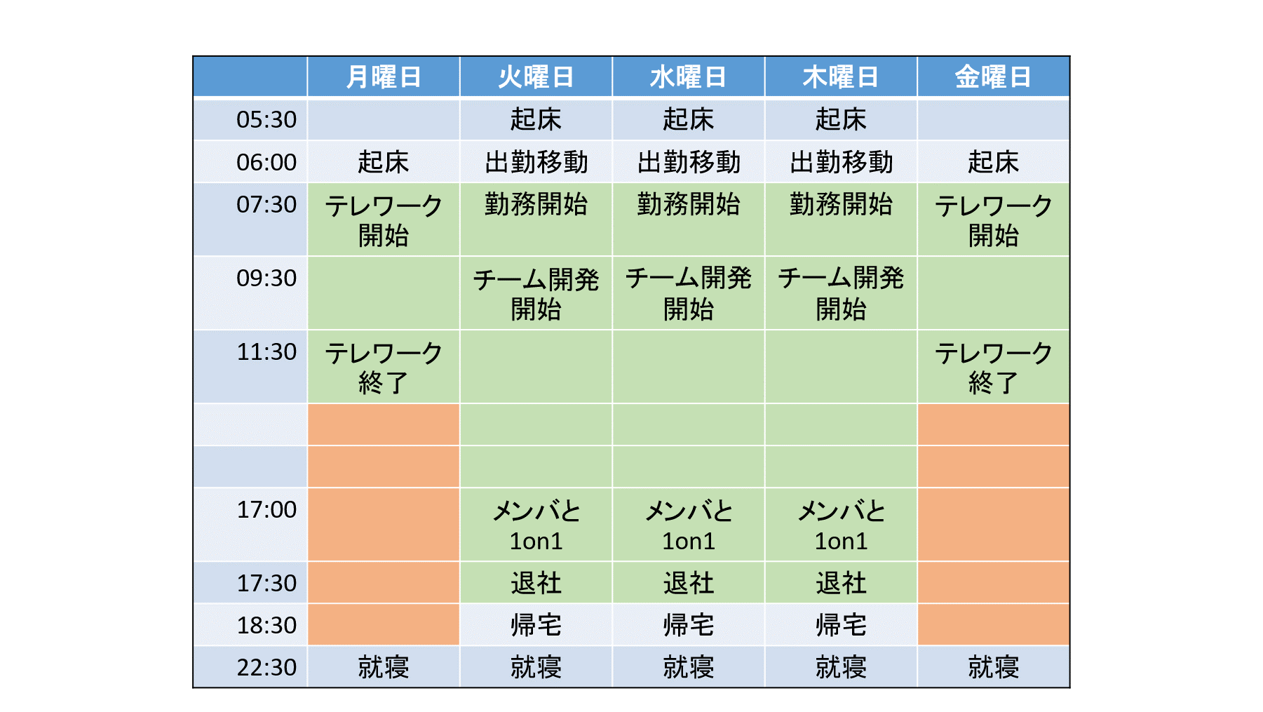
- 投稿日:2020-03-27T10:10:47+09:00
PythonでGoogleカレンダーのfaviconみたいな画像をたくさん生成してVueのプロジェクトに組み込んでみた
この記事は株式会社クロノスの「~2020年春~勝手にやりますアドベントカレンダー」の19日目の記事です。
はじめに
Googleカレンダーのfaviconをご存知でしょうか?
この画像は3月15日に取った画像ですが、実はアクセスした日によって中の数字が変わる仕組みになってたりします。
ということで自分も前にカレンダー的なアプリを作ったのでそれに導入してみることにします。
前まではこんな感じでした。
はい、デフォルトです。
めっちゃVue.jsで作ってます!!!!っていうのが伝わる感じになっていますね。
技術のアピールは大事ですが、アプリとしては若干かっこ悪いので修正してみます。開発者ツールでGoogleカレンダーを見てみると、1〜31まで全パターンのfaviconを用意しているみたいなので、Googleにならって全パターン用意して表示を切り替えるような感じにしてみます。
画像を用意する
使用したツール等
- Google Colaboratory
- Python 3.6.9(Colaboratoryに入ってたバージョン)
- PIL(Python Image Library)
- ICOOON MONO(アイコン)
ベースとなる画像を用意する
今回はICOOON MONOにあるカレンダーのアイコンに数字を重ねて画像を生成してみます。
こちらのアイコンを使用させていただきました。
サイズは48×48、カラーはアプリのテーマに合わせて紫(rgb(121, 88, 214))にしました。
Colaboratoryを開く
以下の画像のような状態にします。
まずベース画像をアップロードします。今回はbase.pngという名前でアップロードしました。
次に加工後の画像を格納するフォルダを作成します。今回はoutというフォルダを作成しました。以上の準備ができたらPythonのコードを書いていきます。
真ん中に数字を配置するためにちょっとトリッキーなことやってたりします。画像を合成するコードfrom PIL import Image # 各種設定 IMAGE_WIDTH = 48 IMAGE_HEIGHT = 48 THEME_COLOR = (121, 88, 214) # 1〜31までループして作成する for i in range(1, 32): # faviconに表示する数字 i_str = str(i) # Font名、サイズを設定する fnt = ImageFont.truetype('LiberationMono-BoldItalic', 25) # 数字を配置する場所を計算するために文字の横幅、縦幅を取得する w, h = fnt.getsize(i_str) # ベースの画像を読み込む im = Image.open('./base.png') draw = ImageDraw.Draw(im) # 読み込んだ画像にテキストを合成する draw.text( # こう書くと真ん中に配置できるみたい(高さだけ3px微調整してます) xy=((IMAGE_WIDTH - w) / 2, (IMAGE_HEIGHT - h) / 2 + 3 ), text=i_str, fill=THEME_COLOR, font=fnt ) # 保存 ./out/favicon01.pngみたいなファイル名にしています im.save("./out/favicon{}.png".format(i_str.zfill(2)))ちなみにフォントは好きなものをダウンロードしてCalaboratoryにアップロードすれば使えるようになりますが、以下のコードを実行すると組み込まれているフォントを確認できます。
今回は数値を扱うだけだったので組み込みのものを使用しました。Colaboratoryのフォントを確認するコードimport subprocess res = subprocess.check_output("fc-list") print(str(res).replace(":", "\n"))上手く行けばoutフォルダ内に以下のような画像が生成されるはずです。
outフォルダ内の画像をダウンロードしましょう。
Colaboratoryだとフォルダ丸ごとダウンロードできなさそうなので
以下のコードでzipにしておくと楽にダウンロードできます。outフォルダをzipに固めるimport shutil shutil.make_archive('./out', 'zip', root_dir='./out')Vueのプロジェクトに組み込む
Vueのプロジェクトのpublicフォルダ内に生成した画像を配置しましょう。
index.htmlを修正します。
faviconを設定しているlinkタグのhref属性を書き換えるscriptを追加します。index.html<!DOCTYPE html> <html lang="ja"> <head> <meta charset="utf-8"> <meta http-equiv="X-UA-Compatible" content="IE=edge"> <meta name="viewport" content="width=device-width,initial-scale=1.0"> <link rel="icon" href="<%= BASE_URL %>favicon.ico"> <!-- 追加部分 --> <script> const faviconLink = document.querySelector("link[rel='icon']"); // 0埋めした日付を取得して favicon01.png みたいな文字列を生成してます faviconLink.href = `favicon${("0" + new Date().getDate()).slice(-2)}.png` </script> <link rel="stylesheet" href="https://use.fontawesome.com/releases/v5.2.0/css/all.css"> <title><%= htmlWebpackPlugin.options.title %></title> </head> <body> <noscript> <strong>We're sorry but <%= htmlWebpackPlugin.options.title %> doesn't work properly without JavaScript enabled. Please enable it to continue.</strong> </noscript> <div id="app"></div> <!-- built files will be auto injected --> </body> </html>いい感じになりました。(満足)
あとはビルドして本番環境にデプロイです。
めでたしめでたし・・・と思いきや・・・
次の日(16日)にアクセスしてみると、アイコンが15から変わってないじゃないですか。
なんでや…!と思い、トランスパイルされたindex.htmlを見てみるとdist/index.html<!DOCTYPE html><html lang=ja><head><meta charset=utf-8><meta http-equiv=X-UA-Compatible content="IE=edge"><meta name=viewport content="width=device-width,initial-scale=1"><link rel=icon href=/favicon.ico><script>const faviconLink = document.querySelector("link[rel='icon']"); これ → faviconLink.href = `favicon15.png`</script><link rel=stylesheet href=https://use.fontawesome.com/releases/v5.2.0/css/all.css><title>ad-calendar</title><link href=/css/app.9c57fa73.css rel=preload as=style><link href=/css/chunk-vendors.a4393e1d.css rel=preload as=style><link href=/js/app.ed32e83e.js rel=preload as=script><link href=/js/chunk-vendors.80e1df9b.js rel=preload as=script><link href=/css/chunk-vendors.a4393e1d.css rel=stylesheet><link href=/css/app.9c57fa73.css rel=stylesheet></head><body><noscript><strong>We're sorry but ad-calendar doesn't work properly without JavaScript enabled. Please enable it to continue.</strong></noscript><div id=app></div><script src=/js/chunk-vendors.80e1df9b.js></script><script src=/js/app.ed32e83e.js></script></body></html>なんとビルドを実行した日付に固定されてしまってますね。
index.html内でJavaScriptのテンプレート記法を使うと実行時の値に固定されてしまうっぽいです。最終的には以下のように修正すると期待通り動作するようになりました。
<!DOCTYPE html> <html lang="ja"> <head> <meta charset="utf-8"> <meta http-equiv="X-UA-Compatible" content="IE=edge"> <meta name="viewport" content="width=device-width,initial-scale=1.0"> <link rel="icon" href="<%= BASE_URL %>favicon.ico"> <script> const faviconLink = document.querySelector("link[rel='icon']"); // 変数に格納するようにした const now = new Date(); const nowDate = ("0" + now.getDate()).slice(-2); // +演算子で文字列結合する faviconLink.href = "<%= BASE_URL %>favicon" + nowDate + ".png"; </script> <link rel="stylesheet" href="https://use.fontawesome.com/releases/v5.2.0/css/all.css"> <title><%= htmlWebpackPlugin.options.title %></title> </head> <body> <noscript> <strong>We're sorry but <%= htmlWebpackPlugin.options.title %> doesn't work properly without JavaScript enabled. Please enable it to continue.</strong> </noscript> <div id="app"></div> <!-- built files will be auto injected --> </body> </html>参考
https://qiita.com/agajo/items/90a29627e7c9a06ec24a
https://www.tech-tech.xyz/drawtext.html
https://icooon-mono.com/license/
https://stackoverflow.com/questions/1970807/center-middle-align-text-with-pil