- 投稿日:2020-03-21T22:03:57+09:00
(今さら)GeForce GTX960でGPUのDeep Learning環境構築
はじめに
最近ほとんど使っていなかった自作デスクトップPCに、NVIDIA製のGPU(GeForce GTX960)が入っているのを思い出し、折角なのでこれを活用してDeep Learningが出来る環境を構築してみようと思いやってみました。
5年前に購入したGPUにも関わらず、処理速度が段違いに速くGPUの素晴らしさに驚きました(笑)
msi GeForce GTX960 Gaming 2G MGSV環境
- Windows 10 Pro (Version 1909)
- Python 3.6.4 (Anaconda3 5.1.0)
必要なもの
- NVIDIA製のGPU
- Tensorflow-gpu
- Keras
- Microsoft Visual Studio C++ (MSVC)
- NVIDIA Driver
- CUDA
- cuDNN
バージョン確認
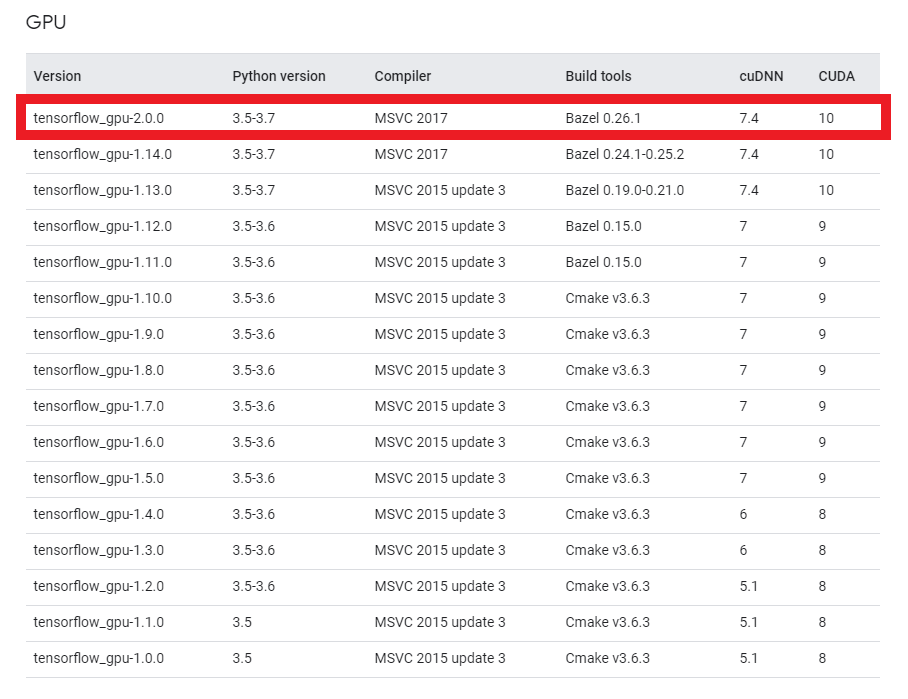
GPU環境でTensorflow/Kerasを使用するには、上記必要なものをそれぞれ対応するバージョンで合わせなければなりません。
Tensorflowのサイトにマッチングテーブルがありますので、必ず確認して下さい。
基本的には、Tensorflowのバージョンに合わせてそれぞれ対応するバージョンをインストールすれば良いと思います。
何か理由があってバージョン指定がなければ最新でOKです。
投稿時点(2020/03/21)では2.0.0が最新なので、2.0.0で構築します。
Conda環境作成&Tensorflow-gpuインストール
TensorflowのCPU版とGPU版が混在していると、CPU版が自動的に選択されるみたいなので新しく環境を作ります。
cmd> conda create -n tf200gpu Python=3.6.4作成完了したら、環境を有効化してTensorflow-gpuをインストールします。
cmd> conda activate tf200gpu (tf200gpu)> pip install tensorflow-gpu==2.0.0↓このエラーが出る場合は以下記事を参照
ERROR: cannot uninstall 'wrapt'. It is a distutils installed project and thus we cannot accurately determine which files belong to it which would lead to only a partial uninstall.インストール完了したら、
pip listで以下内容を確認して下さい。
(この段階でPythonでimport tensorflowを実行しても、CUDA/cuDNNが入っていないのでエラーになります)
- CPU版Tensorflowがインストールされていないか?
- Tensorflow-gpuがインストールされていて、バージョンは2.0.0か?
Kerasのインストール
Kerasは特に問題無くインストール出来ると思います。僕の環境ではバージョン2.3.1が入りました。
cmd(tf200gpu)> pip install kerasTensorflow同様、
pip listでインストールが出来ているか確認して下さい。Visual Studio C++2017のインストール
TensorflowのバージョンとマッチしたVisual StudioをMicrosoftのダウンロードサイトから入手してインストールします。
今回は2017になりますので、Visual Studio Community 2017をインストール。
インストール時に「C++ ワークロードを使用したデスクトップ開発」にチェックを入れて下さい。
(結構時間かかる…)
NVIDIA Driverのインストール
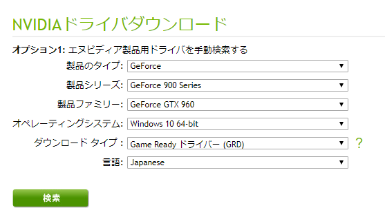
NVIDIAのダウンロードサイトから、製品を選択してインストーラを入手。他のグラフィックボードの場合は、適宜変えて下さい。
特別なことは何もせず、「次に」を押し続けていれば問題無くインストール完了するはずです。CUDAのインストール
CUDAはNVIDIAが開発・提供している、GPU向けの汎用並列コンピューティングプラットフォームです。
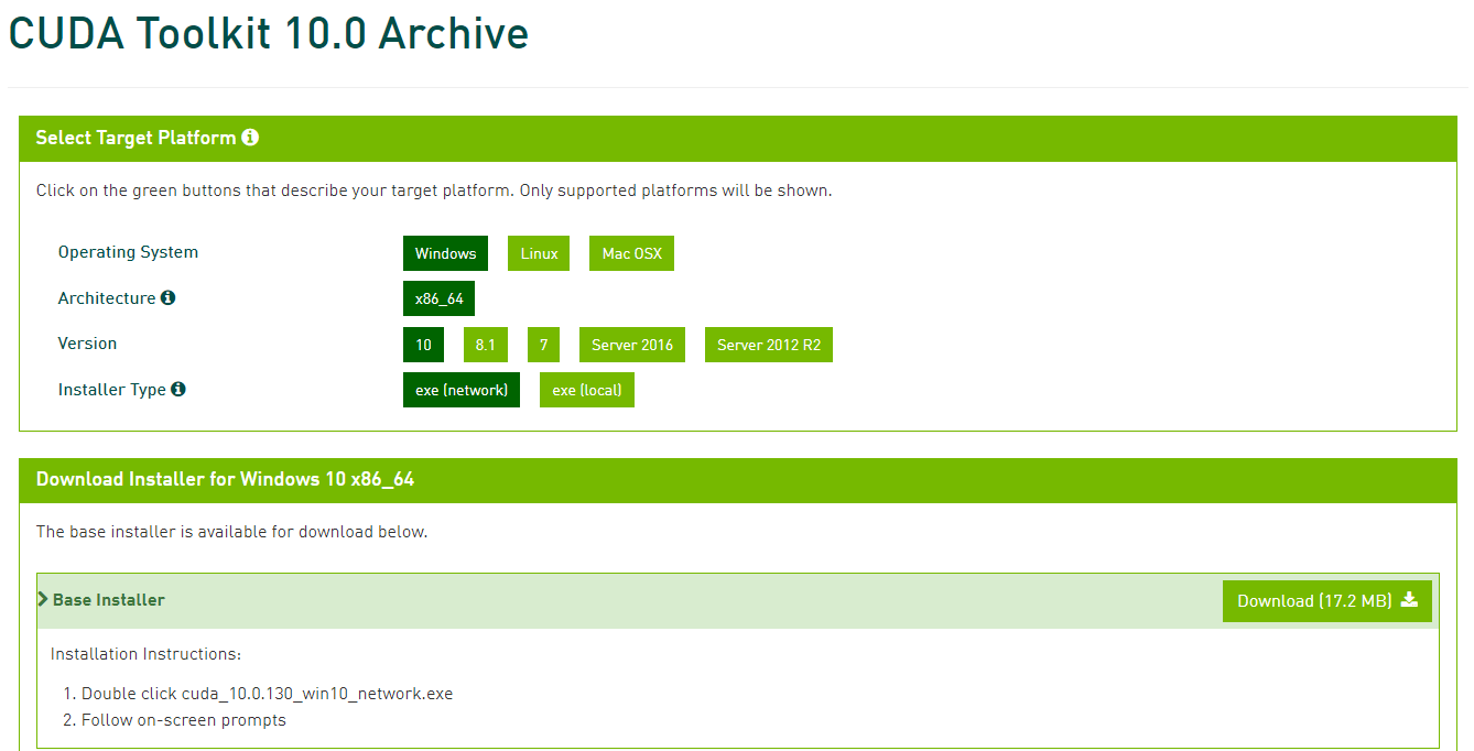
CUDA Toolkitのダウンロードサイトからインストーラを入手してインストールします。
インストーラを入手するのに無料アカウントの作成が必要なので、ちゃちゃっと作ります。
今回はCUDA Toolkit 10.0をインストールします。OSの種類やバージョンを選んで、exe(network)を選択します。
(ネット接続出来ないPCにインストールする場合はlocalを選んで下さい)
ダウンロードが終わったら、インストーラを起動し、Driver同様に「次に」を押し続ければインストール出来ます。
cuDNNのインストール
続いてNVIDAが公開するDeep Learning用のライブラリであるcuDNNをインストールします。
こちらもアカウントが必要になりますので、CUDAの時に作ったアカウントでログインして下さい。
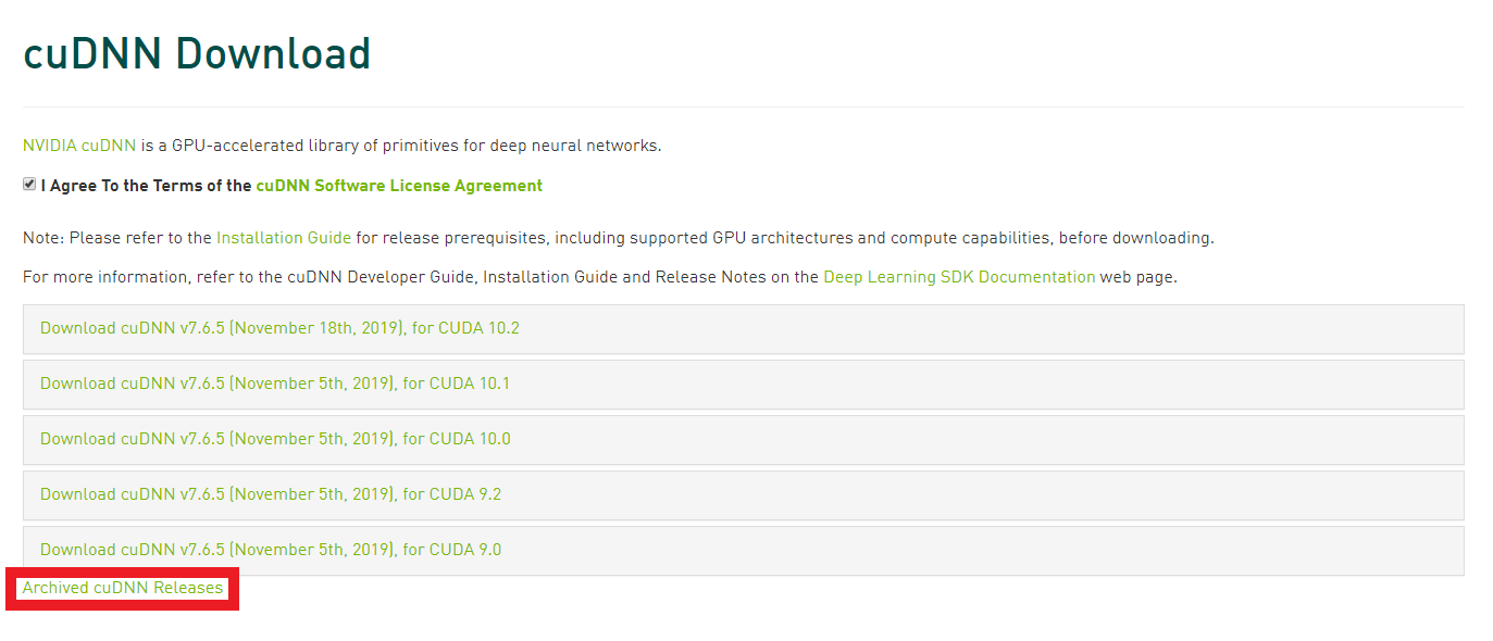
今回は、7.4.2 for CUDA 10をcuDNNのダウンロードサイトから入手します。
「I Agree To the Terms of the cuDNN Software License Agreement」にチェックを入れると、いくつか選択肢が出てきます。この中に欲しいバージョンが無ければ、赤枠の「Archived cuDNN Releases」をクリックすれば過去のリリースが出てきます。
ダウンロードしたzipを解凍すると、bin、include、libの3つのフォルダと、NVIDIA_SLA_cuDNN_Support.txtというテキストファイルがあると思います。
Windows ExplorerでC:\Program Files\NVIDIA GPU Computing Toolkit\CUDA\v.10.0を開き、そこにも同様にbin、include、libのフォルダが存在しますので、ダウンロードしたフォルダの中身をそれぞれ同じ名前のフォルダ内にコピペすることでインストール完了です。
管理者権限を求められることがありますので、許可してあげて下さい。GPUが認識されているか確認
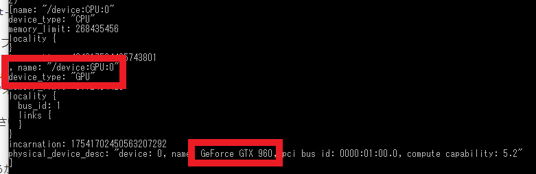
以上でインストール系は完了です。GPUがちゃんと認識されているかを確認するためにコマンドプロンプトで以下を実行してみます。
cmd(tf200gpu)> python -c "from tensorflow.python.client import device_lib;print(device_lib.list_local_devices())"ちゃんと認識されている…!!
いざ実行!
では早速Tensorflow-gpuを使って学習させてみる…も以下エラーに阻まれた。
tensorflow.python.framework.errors_impl.UnknownError: Failed to get convolution algorithm. This is probably because cuDNN failed to initialize, so try looking to see if a warning log message was printed above.こちらの記事を参考にしたところ、cudatooklitもcudnnもcondaのlistに出てこない…
ので、conda install cudnnしてみたら候補が出てきたので、インストールしてみる。
ちなみに、conda install cudnnで、cudatoolkitもcudnnもインストール出来るみたいです。
上記でインストールしたの:
- cudatoolkit 10.2.89
- cudnn 7.6.5
再度学習のコードを実行してみたら、GPUで問題無く動作するようになりました!!
CUDAとcuDNNは2回インストールしているので、これが正しい方法かはわかりませんが(しかもバージョン違うし)とりあえずは動いているので良しとします(笑)
今後何か問題が出たり、正しい方法がわかったら記事更新します!
(詳しい方、コメントで教えて下さい~(´;ω;`))結果
某オンライン研修プログラムで作った以下学習用のPythonコードで測定してみます。
入力された画像をCNNを用いて3つのクラスに分類する画像認識プログラムの学習コードです。
学習用の画像データは、事前に.npy形式で保存してあるものをロードします。
50×50ピクセルの画像を157枚(中途半端)、バッチサイズ32、エポック100で学習させてみたところ…
Processor Time CPU 0:01:22.239975 GPU 0:00:15.542190 GPUの方が約5.4倍速いですね。
(ちなみに搭載CPUはIntel Core i5-6600K @ 3.5GHzです)train.pyimport keras from keras.models import Sequential from keras.layers import Conv2D, MaxPooling2D from keras.layers import Activation, Dropout, Flatten, Dense from keras.utils import np_utils import numpy as np import datetime classes = ["class1", "class2", "class3"] num_classes = len(classes) image_size = 50 def main(): X_train, X_test, y_train, y_test = np.load("./data.npy", allow_pickle=True) X_train = X_train.astype("float") / 256 X_test = X_test.astype("float") / 256 y_train = np_utils.to_categorical(y_train, num_classes) y_test = np_utils.to_categorical(y_test, num_classes) model = model_train(X_train, y_train) model_eval(model, X_test, y_test) def model_train(X, y): model = Sequential() model.add(Conv2D(32, (3, 3), padding='same', input_shape=X.shape[1:])) model.add(Activation('relu')) model.add(Conv2D(32, (3, 3))) model.add(Activation('relu')) model.add(MaxPooling2D(pool_size=(2, 2))) model.add(Dropout(0.25)) model.add(Conv2D(64, (3, 3), padding='same')) model.add(Activation('relu')) model.add(Conv2D(64, (3, 3))) model.add(Activation('relu')) model.add(MaxPooling2D(pool_size=(2, 2))) model.add(Dropout(0.25)) model.add(Flatten()) model.add(Dense(512)) model.add(Activation('relu')) model.add(Dropout(0.5)) model.add(Dense(3)) model.add(Activation('softmax')) opt = keras.optimizers.adam(lr=0.0001, decay=1e-6) model.compile( loss='categorical_crossentropy', optimizer=opt, metrics=['accuracy'] ) model.fit(X, y, batch_size=32, epochs=100) return model def model_eval(model, X, y): scores = model.evaluate(X, y, verbose=1) print('Test Loss: ', scores[0]) print('Test Accuracy: ', scores[1]) if __name__ == "__main__": start_time = datetime.datetime.now() main() end_time = datetime.datetime.now() print("Time: " + str(end_time - start_time))

- 投稿日:2020-03-21T18:34:16+09:00
Elasticsearchで類似ベクトル探索 / 類似画像検索 [TensorFlowでDeep Learning 20]
(目次はこちら)
はじめに
3年ほど前に、Deep FeaturesとFaissというタイトルで画像検索に関して書いたが、2020年3月AWSから、Build k-Nearest Neighbor (k-NN) similarity search engine with Amazon Elasticsearch Serviceが発表されたことを教えてもらい飛びついた。しかもただただサポートされているだけじゃなくて、HNSWで実装されているとのこと。
Built using the lightweight and efficient Non-Metric Space Library (NMSLIB), k-NN enables high scale, low latency nearest neighbor search on billions of documents across thousands of dimensions with the same ease as running any regular Elasticsearch query.
類似ベクトル探索/類似画像検索をElasticsearchで、しかもマネージドサービスで提供できるのは非常にメリットが大きくて、いろいろな用途で使いたい。この記事は、このサービスがすぐにでも実用できるものなのか確認したときの記録です。
(Python: 3.6.8, Tensorflow: 2.1.0で動作確認済み)
前提条件
この条件で、1クエリあたり、10ms〜20msで返ってくるなら、いろいろ用途がありそう
- ベクトル次元: 1,000〜
- ベクトル数: 1,000,000〜
- サーバスペック: AWS ec2 r5.large (2コア, 16GBメモリ) 1台
データ
若干重複はあるもののDeepFashionとDeepFashion2を合わせると約百万件(991,257)
特徴ベクトル抽出
簡単に、MobileNetV2のImageNetのPre-trained modelを使う。ベクトルは1,280次元。
import struct
import glob
import numpy as np
import tensorflow as tf
from tensorflow.keras.applications.mobilenet_v2 import preprocess_input
import tensorflow.keras.layers as layers
from tensorflow.keras.models import Model

def preprocess(img_path, input_shape):
    img = tf.io.read_file(img_path)
    img = tf.image.decode_jpeg(img, channels=input_shape[2])
    img = tf.image.resize(img, input_shape[:2])
    img = preprocess_input(img)
    return img

def main():
    batch_size = 100
    input_shape = (224, 224, 3)
    base = tf.keras.applications.MobileNetV2(input_shape=input_shape,
                                             include_top=False,
                                             weights='imagenet')
    base.trainable = False
    model = Model(inputs=base.input, outputs=layers.GlobalAveragePooling2D()(base.output))

    fnames = glob.glob('deepfashion*/**/*.jpg', recursive=True)
    list_ds = tf.data.Dataset.from_tensor_slices(fnames)
    ds = list_ds.map(lambda x: preprocess(x, input_shape), num_parallel_calls=-1)
    dataset = ds.batch(batch_size).prefetch(-1)

    with open('fvecs.bin', 'wb') as f:
        for batch in dataset:
            fvecs = model.predict(batch)

            fmt = f'{np.prod(fvecs.shape)}f'
            f.write(struct.pack(fmt, *(fvecs.flatten())))

    with open('fnames.txt', 'w') as f:
        f.write('\n'.join(fnames))

if __name__ == '__main__':
    main()
事前検証
Faissにも、HNSWが実装されているので、パラメータ選定の意味も含めて動作検証を行う。
Amazon Elasticsearch Serviceでは、コサイン類似度でスコアが返ってくるので、ここでも、normalize()して、L2をコサイン類似度に変換している。import os import time import math import random import numpy as np import json from sklearn.preprocessing import normalize import faiss def dist2sim(d): return 1 - d / 2 def get_index(index_type, dim): if index_type == 'hnsw': m = 48 index = faiss.IndexHNSWFlat(dim, m) index.hnsw.efConstruction = 128 return index elif index_type == 'l2': return faiss.IndexFlatL2(dim) raise def populate(index, fvecs, batch_size=1000): nloop = math.ceil(fvecs.shape[0] / batch_size) for n in range(nloop): s = time.time() index.add(normalize(fvecs[n * batch_size : min((n + 1) * batch_size, fvecs.shape[0])])) print(n * batch_size, time.time() - s) return index def main(): dim = 1280 fvec_file = 'fvecs.bin' index_type = 'hnsw' #index_type = 'l2' index_file = f'{fvec_file}.{index_type}.index' fvecs = np.memmap(fvec_file, dtype='float32', mode='r').view('float32').reshape(-1, dim) if os.path.exists(index_file): index = faiss.read_index(index_file) if index_type == 'hnsw': index.hnsw.efSearch = 256 else: index = get_index(index_type, dim) index = populate(index, fvecs) faiss.write_index(index, index_file) print(index.ntotal) q_idx = [random.randint(0, fvecs.shape[0]) for _ in range(100)] k = 10 s = time.time() dists, idxs = index.search(normalize(fvecs[q_idx]), k) print((time.time() - s) / len(q_idx)) print(idxs[0], dist2sim(dists[0])) s = time.time() for i in q_idx: dists, idxs = index.search(normalize(fvecs[i:i+1]), k) print((time.time() - s) / len(q_idx)) if __name__ == '__main__': main()検索時間
HNSWすばらしい。これがElasticsearchで実現できるとステキ。
Batch Search Single Query Search IndexFlatL2 110 ms/image 530 ms/image IndexHNSWFlat 0.9 ms/image 5 ms/image 類似画像検索結果
最左列がクエリ画像で、右側の列が、類似度が高い順に10画像。
上記、HNSWのパラメータ(m=48, efConstruction=128, efSearch=256)で、今回の検証に耐えうるReallが出てると判断(厳密な検証はしていない)。
ImageNetのPre-trained modelでここまでいけるんだと感心。
Amazon Elasticsearch Service
AWSのコンソールからポチポチやって、10分くらい待つとインスタンスが立ち上がる。
データ挿入
import time
import math
import numpy as np
import json
import certifi
from elasticsearch import Elasticsearch, helpers
from sklearn.preprocessing import normalize

dim = 1280
fvecs = np.memmap('fvecs.bin', dtype='float32', mode='r').view('float32').reshape(-1, dim)

idx_name = 'imsearch'
es = Elasticsearch(hosts=['https://vpc-xxxxxxxxxxx.us-west-2.es.amazonaws.com'],
                   ca_certs=certifi.where())

mapping = {
    "settings" : {
        "index" : {
            "knn": True,
            "knn.algo_param" : {
                "ef_search" : "256",
                "ef_construction" : "128",
                "m" : "48"
            }
        }
    },
    'mappings': {
        'properties': {
            'fvec': {
                'type': 'knn_vector',
                'dimension': dim
            }
        }
    }
}

res = es.indices.create(index=idx_name, body=mapping, ignore=400)
print(res)

bs = 200
nloop = math.ceil(fvecs.shape[0] / bs)
for k in range(nloop):
    rows = [{'_index': idx_name, '_id': f'{i}',
             '_source': {'fvec': normalize(fvecs[i:i+1])[0].tolist()}}
             for i in range(k * bs, min((k + 1) * bs, fvecs.shape[0]))]
    s = time.time()
    helpers.bulk(es, rows, request_timeout=30)
    print(k, time.time() - s)
1時間くらい待つと、Searchable Documentsがデータ件数と同じに。
res = es.cat.indices(v=True)
print(res)
health status index uuid pri rep docs.count docs.deleted store.size pri.store.size yellow open imsearch 2fvSq3doQ5-4EHhpI_NfhA 5 1 991257 0 24.8gb 24.8gb検索
k = 10
res = es.search(request_timeout=30, index=idx_name,
                body={'size': k, '_source': False,
                      'query': {'knn': {'fvec': {'vector': normalize(fvecs[0:1])[0].tolist(), 'k': k}}}})
print(json.dumps(res, indent=2))
目を疑う結果に。。。Warmupしても同じ。。。 1クエリあたり15s
サーバ台数を3台にしても現実的なレスポンス時間は得られず。
Faissを使った検証と同じドキュメントが返ってきていることは確認できた。{ "took": 15471, "timed_out": false, "_shards": { "total": 5, "successful": 5, "skipped": 0, "failed": 0 }, "hits": { "total": { "value": 1203, "relation": "eq" }, "max_score": 1.0, "hits": [ { "_index": "imsearch", "_type": "_doc", "_id": "340460", "_score": 1.0 }, { "_index": "imsearch", "_type": "_doc", "_id": "355432", "_score": 0.6760856 }, ...あとがき
Amazon Elasticsearch Serviceにデータを入れるところまではよかったが、現実的なレスポンス時間を得ることはできず。何か間違っているんだろうか、、、わからない。。。


- 投稿日:2020-03-21T18:34:16+09:00
Elasticsearchで類似ベクトル探索 / 類似画像検索
(目次はこちら)
はじめに
3年ほど前に、Deep FeaturesとFaissというタイトルで画像検索に関して書いたが、2020年3月AWSから、Build k-Nearest Neighbor (k-NN) similarity search engine with Amazon Elasticsearch Serviceが発表されたことを教えてもらい飛びついた。しかもただただサポートされているだけじゃなくて、HNSWで実装されているとのこと。
Built using the lightweight and efficient Non-Metric Space Library (NMSLIB), k-NN enables high scale, low latency nearest neighbor search on billions of documents across thousands of dimensions with the same ease as running any regular Elasticsearch query.
類似ベクトル探索/類似画像検索をElasticsearchで、しかもマネージドサービスで提供できるのは非常にメリットが大きくて、いろいろな用途で使いたい。この記事は、このサービスがすぐにでも実用できるものなのか確認したときの記録です。
(Python: 3.6.8, Tensorflow: 2.1.0で動作確認済み)
前提条件
この条件で、1クエリあたり、10ms〜20msで返ってくるなら、いろいろ用途がありそう
- ベクトル次元: 1,000〜
- ベクトル数: 1,000,000〜
- サーバスペック: AWS ec2 r5.large (2コア, 16GBメモリ) 1台
データ
若干重複はあるもののDeepFashionとDeepFashion2を合わせると約百万件(991,257)
特徴ベクトル抽出
簡単に、MobileNetV2のImageNetのPre-trained modelを使う。ベクトルは1,280次元。
import struct
import glob
import numpy as np
import tensorflow as tf
from tensorflow.keras.applications.mobilenet_v2 import preprocess_input
import tensorflow.keras.layers as layers
from tensorflow.keras.models import Model

def preprocess(img_path, input_shape):
    img = tf.io.read_file(img_path)
    img = tf.image.decode_jpeg(img, channels=input_shape[2])
    img = tf.image.resize(img, input_shape[:2])
    img = preprocess_input(img)
    return img

def main():
    batch_size = 100
    input_shape = (224, 224, 3)
    base = tf.keras.applications.MobileNetV2(input_shape=input_shape,
                                             include_top=False,
                                             weights='imagenet')
    base.trainable = False
    model = Model(inputs=base.input, outputs=layers.GlobalAveragePooling2D()(base.output))

    fnames = glob.glob('deepfashion*/**/*.jpg', recursive=True)
    list_ds = tf.data.Dataset.from_tensor_slices(fnames)
    ds = list_ds.map(lambda x: preprocess(x, input_shape), num_parallel_calls=-1)
    dataset = ds.batch(batch_size).prefetch(-1)

    with open('fvecs.bin', 'wb') as f:
        for batch in dataset:
            fvecs = model.predict(batch)

            fmt = f'{np.prod(fvecs.shape)}f'
            f.write(struct.pack(fmt, *(fvecs.flatten())))

    with open('fnames.txt', 'w') as f:
        f.write('\n'.join(fnames))

if __name__ == '__main__':
    main()
事前検証
Faissにも、HNSWが実装されているので、パラメータ選定の意味も含めて動作検証を行う。
Amazon Elasticsearch Serviceでは、コサイン類似度でスコアが返ってくるので、ここでも、normalize()して、L2をコサイン類似度に変換している。import os import time import math import random import numpy as np import json from sklearn.preprocessing import normalize import faiss def dist2sim(d): return 1 - d / 2 def get_index(index_type, dim): if index_type == 'hnsw': m = 48 index = faiss.IndexHNSWFlat(dim, m) index.hnsw.efConstruction = 128 return index elif index_type == 'l2': return faiss.IndexFlatL2(dim) raise def populate(index, fvecs, batch_size=1000): nloop = math.ceil(fvecs.shape[0] / batch_size) for n in range(nloop): s = time.time() index.add(normalize(fvecs[n * batch_size : min((n + 1) * batch_size, fvecs.shape[0])])) print(n * batch_size, time.time() - s) return index def main(): dim = 1280 fvec_file = 'fvecs.bin' index_type = 'hnsw' #index_type = 'l2' index_file = f'{fvec_file}.{index_type}.index' fvecs = np.memmap(fvec_file, dtype='float32', mode='r').view('float32').reshape(-1, dim) if os.path.exists(index_file): index = faiss.read_index(index_file) if index_type == 'hnsw': index.hnsw.efSearch = 256 else: index = get_index(index_type, dim) index = populate(index, fvecs) faiss.write_index(index, index_file) print(index.ntotal) q_idx = [random.randint(0, fvecs.shape[0]) for _ in range(100)] k = 10 s = time.time() dists, idxs = index.search(normalize(fvecs[q_idx]), k) print((time.time() - s) / len(q_idx)) print(idxs[0], dist2sim(dists[0])) s = time.time() for i in q_idx: dists, idxs = index.search(normalize(fvecs[i:i+1]), k) print((time.time() - s) / len(q_idx)) if __name__ == '__main__': main()検索時間
HNSWすばらしい。これがElasticsearchで実現できるとステキ。
Batch Search Single Query Search IndexFlatL2 110 ms/image 530 ms/image IndexHNSWFlat 0.9 ms/image 5 ms/image 類似画像検索結果
最左列がクエリ画像で、右側の列が、類似度が高い順に10画像。
上記、HNSWのパラメータ(m=48, efConstruction=128, efSearch=256)で、今回の検証に耐えうるReallが出てると判断(厳密な検証はしていない)。
ImageNetのPre-trained modelでここまでいけるんだと感心。
Amazon Elasticsearch Service
AWSのコンソールからポチポチやって、10分くらい待つとインスタンスが立ち上がる。
データ挿入
import time
import math
import numpy as np
import json
import certifi
from elasticsearch import Elasticsearch, helpers
from sklearn.preprocessing import normalize

dim = 1280
fvecs = np.memmap('fvecs.bin', dtype='float32', mode='r').view('float32').reshape(-1, dim)

idx_name = 'imsearch'
es = Elasticsearch(hosts=['https://vpc-xxxxxxxxxxx.us-west-2.es.amazonaws.com'],
                   ca_certs=certifi.where())

mapping = {
    "settings" : {
        "index" : {
            "knn": True,
            "knn.algo_param" : {
                "ef_search" : "256",
                "ef_construction" : "128",
                "m" : "48"
            }
        }
    },
    'mappings': {
        'properties': {
            'fvec': {
                'type': 'knn_vector',
                'dimension': dim
            }
        }
    }
}

res = es.indices.create(index=idx_name, body=mapping, ignore=400)
print(res)

bs = 200
nloop = math.ceil(fvecs.shape[0] / bs)
for k in range(nloop):
    rows = [{'_index': idx_name, '_id': f'{i}',
             '_source': {'fvec': normalize(fvecs[i:i+1])[0].tolist()}}
             for i in range(k * bs, min((k + 1) * bs, fvecs.shape[0]))]
    s = time.time()
    helpers.bulk(es, rows, request_timeout=30)
    print(k, time.time() - s)
1時間くらい待つと、Searchable Documentsがデータ件数と同じに。
res = es.cat.indices(v=True)
print(res)
health status index uuid pri rep docs.count docs.deleted store.size pri.store.size yellow open imsearch 2fvSq3doQ5-4EHhpI_NfhA 5 1 991257 0 24.8gb 24.8gb検索
k = 10
res = es.search(request_timeout=30, index=idx_name,
                body={'size': k, '_source': False,
                      'query': {'knn': {'fvec': {'vector': normalize(fvecs[0:1])[0].tolist(), 'k': k}}}})
print(json.dumps(res, indent=2))
目を疑う結果に。。。Warmupしても同じ。。。 1クエリあたり15s
サーバ台数を3台にしても現実的なレスポンス時間は得られず。
Faissを使った検証と同じドキュメントが返ってきていることは確認できた。{ "took": 15471, "timed_out": false, "_shards": { "total": 5, "successful": 5, "skipped": 0, "failed": 0 }, "hits": { "total": { "value": 1203, "relation": "eq" }, "max_score": 1.0, "hits": [ { "_index": "imsearch", "_type": "_doc", "_id": "340460", "_score": 1.0 }, { "_index": "imsearch", "_type": "_doc", "_id": "355432", "_score": 0.6760856 }, ...あとがき
Amazon Elasticsearch Serviceにデータを入れるところまではよかったが、現実的なレスポンス時間を得ることはできず。何か間違っているんだろうか、、、わからない。。。
- 投稿日:2020-03-21T16:26:48+09:00
TensorFlow 2.2.0-rc0(CUDA10.2+cuDNN7.6.5)のビルド手順 - Windows10
TensorFlow 2.2.0-rc0(GPU版)をWindows 10でビルドする手順です。
細かい説明は省略して要点だけを記載しているので、もう少し詳しい内容はdev.infohub.ccのBlogなどを参考にしていただければと思います。ビルド環境の準備
ビルドには次の環境を利用します。
CUDAやcuDNN、Pythonなどは事前にPATHを通しておきます。
- CPU: AMD Ryzen Threadripper 3960X
- GPU: NVIDIA TITAN RTX
- Windows 10 Pro 64bit (Ver 1909 build 18363.720)
- CUDA 10.2
- cuDNN 7.6.5
- Visual Studio Community 2019 Ver16.4.6
- Python 3.8.2
- MSYS2
インストールしてC:\msys64\usr\binにパスを通す。- Bazel 2.0.0
ダウンロードしたファイルをbazel.exeにリネームしてパスの通ったフォルダに格納。
※TensorFlow 2.2.0-rc0のビルドに使えるバージョンはBazel 2.0.0だけなので注意!
MSYS2のパッケージ追加
C:\msys64\msys2_shell.cmdを起動して、ビルドに必要なパッケージを追加します。# 必要なパッケージの導入 pacman -S git patch unzip # 以降はMSYS2のコンソールは利用しないので終了 exitTensorFlowのビルド
ビルド用のPython仮想環境
g:\venvs\build_tf2を使ってTensorFlowをビルドしていきます。
パス等はそれぞれの環境に合わせて読み替えてください。以降の操作は、Visual Studio 2019の
x64 Native Tools Command Prompt for VS 2019で起動したコンソール画面を利用します。# 仮想環境を作成して有効化する python -m venv g:\venvs\build_tf2 cd /d g:\venvs\build_tf2 g:\venvs\build_tf2\Scripts\activate.bat # pipのアップグレード(任意) python -m pip install --upgrade pip # ビルドに必要なパッケージを導入 pip install six numpy wheel pip install keras_applications==1.0.8 --no-deps pip install keras_preprocessing==1.1.0 --no-deps # TensorFlow v2.2.0-rc0のソースコードを取得 git clone https://github.com/tensorflow/tensorflow.git cd tensorflow git checkout v2.2.0-rc0 # 不要な環境変数の削除(オプション) # 環境変数全てがパラメータで渡されるため、パラメータの文字列が32768文字を超えると # FATAL: Command line too long (34052 > 32768) というようなエラーが発生する。 # それを防ぐために、ここで不要な環境変数を一時的に削除。 # _OLD_VIRTUAL_PATHは文字数が多くなりがちなので、削除する第一候補。 set _OLD_VIRTUAL_PATH= # ビルド構成の設定 #---------------------------------------------------------------- # <設定例> # Location of Python : (Default) # ROCm support : (Default = N) # CUDA support : Y # CUDA compute capabilities : 7.5 (詳細はhttps://developer.nvidia.com/cuda-gpusを参照) # Optimization flag : /arch:AVX2 # Override eigen... : (Default = Y) #---------------------------------------------------------------- python ./configure.py # ビルド(CUDA向け) # ビルドが完了するまで、数十分~数時間かかります bazel build --config=opt --config=cuda --define=no_tensorflow_py_deps=true --copt=-nvcc_options=disable-warnings //tensorflow/tools/pip_package:build_pip_package # Wheelパッケージの作成 # g:\tensorflow_pkgフォルダにパッケージを作成する(数分かかる) bazel-bin\tensorflow\tools\pip_package\build_pip_package g:\tensorflow_pkg # これでTensorFlowのビルドが完了。exitで終了。 #---------------------------------------------------------------- # <参考> # Bazelのワークファイルは %UserProfile%_bazel_%UserName% に作成されるので # 不要なら、このフォルダを削除してもOK(20GB程度の容量) #---------------------------------------------------------------- exit新規環境にビルドしたTensorFlowを導入
ビルドしたTensorFlowを新しいPythonの仮想環境に導入する方法です。
ここではg:\venvs\tf2に新しい仮想環境を作成する例です。# 仮想環境を作成して有効化 python -m venv g:\venvs\tf2 g:\venvs\tf2\Scripts\activate.bat # pipのアップデート(任意) python -m pip install --upgrade pip # ビルドしたTensorFlowのインストール(作成したwheelファイルを指定するだけ) pip install g:\tensorflow_pkg\tensorflow-2.2.0rc0-cp38-cp38-win_amd64.whl # 動作確認 python -c "import tensorflow as tf; print(tf.__version__); print(tf.keras.__version__)" python -c "import tensorflow as tf; print(tf.reduce_sum(tf.random.normal([1000, 1000])))"備考
TensorFlow 2.2.0-rc0のビルドは、TensorFlow v1の頃に比べると格段に簡単になっている印象を受けます。
今回のビルドでも、python ./configure.pyとしたときに、FATAL: Command line too long (34052 > 32768)というエラーに遭遇しただけで、それ以外は何の問題も発生しませんでした。実行時にDLLが見つからずにエラーになるケースが多くありますが、この場合はCUDA等必要なライブラリへのパスが通っているか確認してみてください。
- 投稿日:2020-03-21T15:13:29+09:00
TensorFlow QuantumでQAOAをやってみる
はじめに
先日発表されたTensorFlow Quantumを触ってみました。
TensorFlowにCirqを統合し、さらに量子回路のパラメーターをニューラルネットで調整する機能をKeras風味で実装した量子機械学習用ライブラリです。公式Tutorialの構成がハードボイルドで、最初に(おそらく実機Qubitを想定した)ゲート回転角誤差の補正計算から入り、次にVQEやQAOAなどのNear term algorithmをすっ飛ばしてMNISTを実装し、結果として現時点では古典NNの方がずっと優れていると結論付けています。
Near term algorithm との親和性が気になるところなので、今回はTensorFlow QuantumでQAOAを試してみます。
また今回の記事内ではQAOAにニューラルネットワークを使うことでパフォーマンスが向上するかといった議論はしませんし、できないと思います。
ニューラルネットワーク構造やハイパーパラメータは特に追い込んでいないため、興味のある方はより良い結果が得られるか色々試すのも良いと思います。題材
題材はこちらの最適化問題をとりあえずそのまま使いました。
公式Tutorial "hello_many_worlds"のコードをベースとしているので、合わせて見ることをおすすめします。実装
ライブラリインポート
import tensorflow as tf
import tensorflow_quantum as tfq

import cirq
import sympy
import numpy as np
from cirq.contrib.svg import SVGCircuit
パラメータ設定
# 変更可能なパラメータ
p = 3 # QAOAのステップ数
K = 20 # 制約条件式のハイパーパラメータ
command_param = 0.1 # ニューラルネットの入力、多分何でも良い

 # Qubit数, 問題によって決まる
N = 6

# QAOA 回転角パラメータをsympy symbolとして用意
control_params = []
for i in range(p):
    gamma = 'gamma' + str(i)
    beta = 'beta' + str(i)
    control_params.append(sympy.symbols(gamma))
    control_params.append(sympy.symbols(beta))
QAOA用ユニタリゲートの用意
元記事の制約条件QUBO式をPauli-Z演算子で構成されたコストハミルトニアンに変換し、時間発展ゲートを実装しました。
ミキサハミルトニアン時間発展と初期状態準備用のゲートも用意しておきます。# コストハミルトニアン時間発展 def CostUnitary(circuit, control_params, i, K): circuit.append(cirq.ZZ(qubits[0], qubits[1])**((K / 2 + 1) * control_params[i])) circuit.append(cirq.ZZ(qubits[0], qubits[2])**(K / 2 * control_params[i])) circuit.append(cirq.Z(qubits[0])**((-K / 2 - 6) * control_params[i])) circuit.append(cirq.ZZ(qubits[1], qubits[2])**((K + 1) / 2 * control_params[i])) circuit.append(cirq.Z(qubits[1])**((- K / 2 - 7) * control_params[i])) circuit.append(cirq.Z(qubits[2])**((- K / 2 - 5) * control_params[i])) circuit.append(cirq.ZZ(qubits[3], qubits[4])**((K / 2 + 1) * control_params[i])) circuit.append(cirq.ZZ(qubits[3], qubits[5])**(K / 2 * control_params[i])) circuit.append(cirq.Z(qubits[3])**((- K / 2 - 6) * control_params[i])) circuit.append(cirq.ZZ(qubits[4], qubits[5])**((K + 1) / 2 * control_params[i])) circuit.append(cirq.Z(qubits[4])**((- K / 2 - 7) * control_params[i])) circuit.append(cirq.Z(qubits[5])**((- K / 2 - 5) * control_params[i])) circuit.append(cirq.ZZ(qubits[0], qubits[3])**(2 * control_params[i])) circuit.append(cirq.ZZ(qubits[0], qubits[4])**(control_params[i])) circuit.append(cirq.ZZ(qubits[1], qubits[3])**(control_params[i])) circuit.append(cirq.ZZ(qubits[1], qubits[4])**(2 * control_params[i])) circuit.append(cirq.ZZ(qubits[1], qubits[5])**(1 / 2 * control_params[i])) circuit.append(cirq.ZZ(qubits[2], qubits[4])**(1 / 2 * control_params[i])) circuit.append(cirq.ZZ(qubits[2], qubits[5])**(2 * control_params[i])) return circuit # ミキサハミルトニアン時間発展 def Mixer(circuit, i, N): for j in range(N): circuit.append(cirq.XPowGate(exponent = control_params[i]).on(qubits[j])) return circuit # 初期状態(|+>)準備 def init_circuit(N): initCircuit = cirq.Circuit() qubits = cirq.GridQubit.rect(1, N) for j in range(N): initCircuit.append(cirq.H(qubits[j])) return initCircuit量子回路生成
上で用意したゲートをQAOAステップ数$p$回作用させます。
init_circuit()は後で使います。qubits = [cirq.GridQubit(i, 0) for i in range(N)] model_circuit = cirq.Circuit() for i in range(p): model_circuit = CostUnitary(model_circuit, control_params, 2 * i, K) model_circuit = Mixer(model_circuit, 2 * i + 1, N)Operator定義
コストハミルトニアンの期待値を目的関数として最適化を行うため、コストハミルトニアンをOperatorとして実装します。
def ZZoperator(i, j):
    return cirq.Z(qubits[i]) * cirq.Z(qubits[j])

operators = [[-1 * ((K / 2 + 1) * ZZoperator(0, 1) + (K / 2) * ZZoperator(0, 2) - \
            (K / 2 + 6) * cirq.Z(qubits[0]) + (K / 2 + 1 / 2) * ZZoperator(1, 2) - \
            (K / 2 + 7) * cirq.Z(qubits[1]) - (K / 2 + 5) * cirq.Z(qubits[2]) + \
            (K / 2 + 1) * ZZoperator(3, 4) + (K / 2) * ZZoperator(3, 5) - \
            (K / 2 + 6) * cirq.Z(qubits[3]) + (K / 2 + 1 / 2) * ZZoperator(4, 5) - \
            (K / 2 + 7) * cirq.Z(qubits[4]) - (K / 2 + 5) * cirq.Z(qubits[5]) + \
            2 * ZZoperator(0, 3) + ZZoperator(0, 4) + ZZoperator(1, 3) + 2 * ZZoperator(1, 4) +\
            1 / 2 * ZZoperator(1, 5) + 1 / 2 * ZZoperator(2, 4) + 2 * ZZoperator(2, 5) + 2 * K + 24)]]
model定義
公式Tutorial "hello_many_worlds"を参考に学習用modelを定義していきます。
controllerには変分パラメータの値を出力するニューラルネットが入ります。
通常のkerasよろしくlayerを追加していきます。commands_inputはcontrollerで組んだニューラルネットの先頭ノードへの入力です。
公式Tutorialでは複数の値を用意し、値によって異なる出力を返すようニューラルネットをトレーニングするなどしています。
今回は1つの値しか使わないため、あまり意味はないです。最後にexpected_outputsを0としています。
この値と実際のコストハミルトニアンの期待値との差を小さくするようにニューラルネットのパラメータが調整されます。expected_outputsはコストハミルトニアン期待値の大域的な最小値(最大値)としたいところですが、予めわかっていない方が一般的じゃないかと思います。
ここをどのような値にするか。今回は0未満の値をとらないQUBO式が与えられているためコストハミルトニアンの期待値も0に向かって最適化しました。# QAOAパラメータ最適化用のネットワークを定義 controller = tf.keras.Sequential([ tf.keras.layers.Dense(20 * p, activation='elu'), tf.keras.layers.Dense(len(control_params)) ]) init_circuits = tfq.convert_to_tensor([init_circuit(N)]) commands_input = tf.keras.layers.Input(shape=(1), dtype=tf.dtypes.float32, name='commands_input') circuits_input = tf.keras.Input(shape=(), # The circuit-tensor has dtype `tf.string` dtype=tf.dtypes.string, name='circuits_input') operators_input = tf.keras.Input(shape=(1,), dtype=tf.dtypes.string, name='operators_input') dense_2 = controller(commands_input) # tf.keras.Sequential full_circuit = tfq.layers.AddCircuit()(circuits_input, append=model_circuit) expectation_output = tfq.layers.Expectation()(full_circuit, symbol_names=control_params, symbol_values=dense_2, operators=operators_input) model = tf.keras.Model( inputs=[circuits_input, commands_input, operators_input], outputs=[expectation_output]) operator_data = tfq.convert_to_tensor(operators) commands = np.array([[command_param] for i in range(len(operators))], dtype=np.float32) expected_outputs = np.array([[0] for i in range(len(operators))], dtype=np.float32)modelコンパイル
optimizer = tf.keras.optimizers.Adam(learning_rate=0.05)
loss = tf.keras.losses.MeanSquaredError()

model.compile(optimizer=optimizer, loss=loss)
学習
history = model.fit(
    x=[init_circuits, commands, operator_data],
    y=expected_outputs,
    epochs=200,
    verbose=1)
コストハミルトニアン期待値、学習済パラメータの表示
print('Expectation value', model([init_circuits, commands, operator_data]))
after_params = controller.predict(np.array([command_param]))[0]
print('after params: ', after_params)
結果のサンプリング
ニューラルネットでパラメータ最適化された量子回路の出力を測定し、状態をサンプリングします。
得られた状態についてコストハミルトニアンの期待値を計算し、期待値最大の状態が今回の問題の最適解となります(元の制約条件式は最小化問題ですがコストハミルトニアンの符号を変えて最大化問題としています)。param_dict = {} for i in range(len(control_params)): param_dict.update([(control_params[i], after_params[i])]) resolver = cirq.ParamResolver(param_dict) simulator = cirq.Simulator() model_circuit.append(cirq.measure(*qubits, key = 'm')) results = simulator.run(model_circuit, resolver, repetitions=100) def calc_cost(state, operator): qubits = [cirq.GridQubit(i, 0) for i in range(len(state))] test_circuit = cirq.Circuit() for i in range(len(state)): if state[i] == '1': test_circuit.append(cirq.X(qubits[i])) else: test_circuit.append(cirq.I(qubits[i])) output_state_vector = cirq.Simulator().simulate(test_circuit).final_state qubit_map={qubits[0]: 0, qubits[1]: 1, qubits[2]: 2, qubits[3]: 3, qubits[4]: 4, qubits[5]: 5} return operator.expectation_from_wavefunction(output_state_vector, qubit_map).real hist = results.histogram(key='m') keys = list(hist.keys()) print('{:6}'.format('state'), '|', '{}'.format('count'), '|', '{}'.format('cost')) for key in keys: binary = '{:0=6b}'.format(key) count = '{:5}'.format(hist[key]) print(binary, '|', count, '|', calc_cost(binary, operators[0][0]))出力結果例
QAOAパラメータ最適化後の状態に対する
- コストハミルトニアン期待値
- QAOAパラメータ
- 100 shots測定して得られた各状態のカウント数と、今回の制約条件式におけるコスト値(0に近いほど最適解に近い)今回の問題では状態"100001"と"001100"が共にコスト=-8で最適解であると事前計算で確認可能です。
最適解以外の状態もそれなりにサンプリングされていますが、最適解がより高い確率でサンプリングされることが望ましいです。Expectation value tf.Tensor([[-22.023201]], shape=(1, 1), dtype=float32) after params: [-0.44315836 1.8975906 0.39658815 -3.8769927 4.8495026 1.8638508 ] state | count | cost 100001 | 2 | -8.0 # 最適解1 001000 | 8 | -24.0 100000 | 7 | -24.0 010010 | 2 | -16.0 000010 | 15 | -24.0 010100 | 1 | -12.0 011000 | 6 | -50.0 001100 | 6 | -8.0 # 最適解2 000001 | 10 | -24.0 000000 | 13 | -40.0 010000 | 12 | -24.0 000011 | 2 | -50.0 000100 | 8 | -24.0 110101 | 1 | -74.0 100100 | 3 | -16.0 100010 | 2 | -12.0 100011 | 1 | -38.0 101011 | 1 | -72.0まとめ
TensorFlow-quantumでQAOAをやるメリットがあるかと考えると、個人的には微妙です。
そもそもcirqを今回初めて触ったのですがドキュメントが公式・非公式ともにQISkitなどと比べるとかなり少ないです。
それに変分量子最適化計算をするだけならニューラルネットはscipy.optimizerのような感じで用意された方が取り回しが良いのではという気もします。本格的に量子深層学習などを実装する場合に真価を発揮するのかもしれませんが、それはハードが追いつかないでしょうしまだ先かなと感じます。
以上、読んで頂きありがとうございました。
- 投稿日:2020-03-21T00:44:02+09:00
Tensorflow-gpu 2.1.0でCUDNN_STATUS_NOT_INITIALIZEDが出る問題
はじめに
Tensorflow2.1.0で遊ぼうと思ったらCUDNN_STATUS_NOT_INITIALIZEDのエラーが出たので、解決方法を書いていきます。
※Tensorflow2.0.0でも同様のエラーが出るかもしれません。環境
- OS :: Windows10 home
- GPU :: NVIDIA RTX2070
- cuDNN :: 7.6
- CUDA :: 10.1
- Python 3.7.6 :: Anaconda custom (64-bit)
- tensorflow :: tensorflow-gpu==2.1.0
環境は以下を参考にして入れました。
https://www.tensorflow.org/install/source#tested_build_configurationsエラー内容
2020-03-21 00:29:53.137414: I tensorflow/stream_executor/platform/default/dso_loader.cc:44] Successfully opened dynamic library cudart64_101.dll
2020-03-21 00:29:55.399548: I tensorflow/stream_executor/platform/default/dso_loader.cc:44] Successfully opened dynamic library nvcuda.dll
2020-03-21 00:29:55.423219: I tensorflow/core/common_runtime/gpu/gpu_device.cc:1555] Found device 0 with properties:
pciBusID: 0000:01:00.0 name: GeForce RTX 2070 computeCapability: 7.5
coreClock: 1.71GHz coreCount: 36 deviceMemorySize: 8.00GiB deviceMemoryBandwidth: 417.29GiB/s
2020-03-21 00:29:55.430144: I tensorflow/stream_executor/platform/default/dso_loader.cc:44] Successfully opened dynamic library cudart64_101.dll
2020-03-21 00:29:55.438727: I tensorflow/stream_executor/platform/default/dso_loader.cc:44] Successfully opened dynamic library cublas64_10.dll
2020-03-21 00:29:55.445024: I tensorflow/stream_executor/platform/default/dso_loader.cc:44] Successfully opened dynamic library cufft64_10.dll
2020-03-21 00:29:55.449169: I tensorflow/stream_executor/platform/default/dso_loader.cc:44] Successfully opened dynamic library curand64_10.dll
2020-03-21 00:29:55.456919: I tensorflow/stream_executor/platform/default/dso_loader.cc:44] Successfully opened dynamic library cusolver64_10.dll
2020-03-21 00:29:55.462110: I tensorflow/stream_executor/platform/default/dso_loader.cc:44] Successfully opened dynamic library cusparse64_10.dll
2020-03-21 00:29:55.473068: I tensorflow/stream_executor/platform/default/dso_loader.cc:44] Successfully opened dynamic library cudnn64_7.dll
2020-03-21 00:29:55.476609: I tensorflow/core/common_runtime/gpu/gpu_device.cc:1697] Adding visible gpu devices: 0
2020-03-21 00:29:55.479345: I tensorflow/core/platform/cpu_feature_guard.cc:142] Your CPU supports instructions that this TensorFlow binary was not compiled to use: AVX2
2020-03-21 00:29:55.484766: I tensorflow/core/common_runtime/gpu/gpu_device.cc:1555] Found device 0 with properties:
pciBusID: 0000:01:00.0 name: GeForce RTX 2070 computeCapability: 7.5
coreClock: 1.71GHz coreCount: 36 deviceMemorySize: 8.00GiB deviceMemoryBandwidth: 417.29GiB/s
2020-03-21 00:29:55.493764: I tensorflow/stream_executor/platform/default/dso_loader.cc:44] Successfully opened dynamic library cudart64_101.dll
2020-03-21 00:29:55.497168: I tensorflow/stream_executor/platform/default/dso_loader.cc:44] Successfully opened dynamic library cublas64_10.dll
2020-03-21 00:29:55.502105: I tensorflow/stream_executor/platform/default/dso_loader.cc:44] Successfully opened dynamic library cufft64_10.dll
2020-03-21 00:29:55.505886: I tensorflow/stream_executor/platform/default/dso_loader.cc:44] Successfully opened dynamic library curand64_10.dll
2020-03-21 00:29:55.510337: I tensorflow/stream_executor/platform/default/dso_loader.cc:44] Successfully opened dynamic library cusolver64_10.dll
2020-03-21 00:29:55.513831: I tensorflow/stream_executor/platform/default/dso_loader.cc:44] Successfully opened dynamic library cusparse64_10.dll
2020-03-21 00:29:55.518574: I tensorflow/stream_executor/platform/default/dso_loader.cc:44] Successfully opened dynamic library cudnn64_7.dll
2020-03-21 00:29:55.522030: I tensorflow/core/common_runtime/gpu/gpu_device.cc:1697] Adding visible gpu devices: 0
2020-03-21 00:29:56.067998: I tensorflow/core/common_runtime/gpu/gpu_device.cc:1096] Device interconnect StreamExecutor with strength 1 edge matrix:
2020-03-21 00:29:56.071564: I tensorflow/core/common_runtime/gpu/gpu_device.cc:1102]      0
2020-03-21 00:29:56.075105: I tensorflow/core/common_runtime/gpu/gpu_device.cc:1115] 0:   N
2020-03-21 00:29:56.078938: I tensorflow/core/common_runtime/gpu/gpu_device.cc:1241] Created TensorFlow device (/job:localhost/replica:0/task:0/device:GPU:0 with 6304 MB memory) -> physical GPU (device: 0, name: GeForce RTX 2070, pci bus id: 0000:01:00.0, compute capability: 7.5)
2020-03-21 00:29:56.930030: I tensorflow/stream_executor/platform/default/dso_loader.cc:44] Successfully opened dynamic library cublas64_10.dll
2020-03-21 00:29:57.220935: I tensorflow/stream_executor/platform/default/dso_loader.cc:44] Successfully opened dynamic library cudnn64_7.dll
2020-03-21 00:29:58.451976: E tensorflow/stream_executor/cuda/cuda_dnn.cc:329] Could not create cudnn handle: CUDNN_STATUS_NOT_INITIALIZED
2020-03-21 00:29:58.455735: E tensorflow/stream_executor/cuda/cuda_dnn.cc:333] Error retrieving driver version: Unimplemented: kernel reported driver version not implemented on Windows
2020-03-21 00:29:58.461795: E tensorflow/stream_executor/cuda/cuda_dnn.cc:329] Could not create cudnn handle: CUDNN_STATUS_NOT_INITIALIZED
2020-03-21 00:29:58.466492: E tensorflow/stream_executor/cuda/cuda_dnn.cc:333] Error retrieving driver version: Unimplemented: kernel reported driver version not implemented on Windows
2020-03-21 00:29:58.472369: F tensorflow/core/kernels/conv_grad_input_ops.cc:1163] Check failed: stream->parent()->GetConvolveBackwardDataAlgorithms( conv_parameters.ShouldIncludeWinogradNonfusedAlgo<T>(stream->parent()), &algorithms)
解決方法
ソースコード
以下のどちらかをソースコードに入れる。
from tensorflow.compat.v1 import ConfigProto
from tensorflow.compat.v1 import InteractiveSession

config = ConfigProto()
config.gpu_options.per_process_gpu_memory_fraction = 0.2
config.gpu_options.allow_growth = True
session = InteractiveSession(config=config)
import tensorflow as tf gpu_devices = tf.config.experimental.list_physical_devices('GPU') for device in gpu_devices: tf.config.experimental.set_memory_growth(device, True)参考
一番下に記載してありました。
https://github.com/tensorflow/tensorflow/issues/24496おわりに
githubのissueを見る限り、RTX2070もしくはRTX2080だと発生するエラーのようです。