- 投稿日:2021-03-01T23:57:05+09:00
【Scanpy, scRNA-seq】ScanpyのUMAPに再現性を持たせる
起きていた問題
Scanpyで描いたUMAPに再現性がない。
予想としてはPCAの部分で相違が生まれていそう。環境
こちらのDockerイメージをスパコンのSingularityコンテナとして利用。
バージョン情報:scanpy==1.7.0 anndata==0.7.5 umap==0.5.1 numpy==1.19.2 scipy==1.5.2 pandas==1.1.3 scikit-learn==0.23.2 statsmodels==0.12.0 python-igraph==0.9.0 louvain==0.7.0 leidenalg==0.8.3,解決方法
#1187で議論されているように、環境変数
OMP_NUM_THREADSを設定し、BLAS librariesが使用するCPU数を制限することで再現性が確保された。import os os.environ['OMP_NUM_THREADS'] = '1' import numpy as np import pandas as pd import scanpy as sc 〜以下省略〜疑問・補足
ローカルのDockerコンテナおよびJupyterLab上では、同様にしても再現性を確保できなかった。
なぜ?また今回は上記の環境変数
OMP_NUM_THREADSのみの指定で再現性が確保されたが、
#313で取り上げられている通り、ハッシュランダム化を無効化する、os.environ['PYTHONHASHSEED'] = '0'についても指定しておいたほうが良さそう。
- 投稿日:2021-03-01T23:47:14+09:00
playwright-pytestで失敗時の動画を撮っておく
まえおき
playwright-pytest を使ってE2Eテストを始める方法については、以前に以下の記事で紹介した。
ここでは、失敗時の画面キャプチャを撮る方法までは書いたが、実際に自動試験スクリプトを書いていると「どうしてそうなった?!」と思うことが稀によくある。(しかも、そんなテストに限って、じっと見張っていると何回やってもpassしたりするw)
不毛すぎるので、見張らなくてもいいようにエビデンス動画を残しておきたいと思うのがエンジニアである。
playwright-pythonで動画を撮る方法
playwright-python には、自動操作中の動画を記録する機能がある。
以下の記事でも言及されているように、
browser.new_context()もしくはbrowser.new_page()の引数にrecord_video_dir: ./videos/のように指定すればいい。
ただ、これはplaywright-pythonの話であり、そのままplaywright-pytestでは運用できない。なぜかというと
- 成功時の動画はべつに要らない
- 失敗時の動画は「ディレクトリに置いてあるのを見ろ」だと面倒なので、Allureレポートに添付したい
(特に2つめの理由が大きい)
playwright-pytest でAllureレポートに失敗時の動画を添付する方法
本題。
動画を撮る
テスト開始時に、そのテストが開始するか失敗するかはわからないので、動画の記録自体は無条件に行う。
playwright-pytestのソースを見ると、new_contextに渡す引数は
browser_context_argsでカスタマイズできるようになっているので、適当にconftest.pyあたりに以下を追加する。@pytest.fixture(scope="session") def browser_context_args(browser_context_args, tmpdir_factory: pytest.TempdirFactory): return { **browser_context_args, "record_video_dir": tmpdir_factory.mktemp('videos') }
record_video_dirは一時ディレクトリを作って、テスト終了後には消える場所にしているのがポイント。テスト失敗時のレポートに動画を添付する
def pytest_runtest_makereport(item, call) -> None:
    if call.when == "call":
        if call.excinfo is not None and "page" in item.funcargs:
            page: Page = item.funcargs["page"]

            # ref: https://stackoverflow.com/q/29929244
            allure.attach(
                page.screenshot(type='png'),
                name=f"{slugify(item.nodeid)}.png",
                attachment_type=allure.attachment_type.PNG
            )

            video_path = page.video.path()
            page.context.close()  # ensure video saved
            allure.attach(
                open(video_path, 'rb').read(),
                name=f"{slugify(item.nodeid)}.webm",
                attachment_type=allure.attachment_type.WEBM
            )
スクリーンショットを撮ったあとの video_path = ... からの処理が動画の記録部分。
Playwrightの動画記録は、BrowserContext#close したタイミングで書き込みが完了されるので、明示的にcloseを読んで動画ファイルを確定させてからattachしているのがポイント。
もし明示的にcloseを呼ばないと、0秒の動画が貼り付けられたり、手順の途中で切れた動画が添付されたりするので注意。Allureレポートでは、以下のように、事象が起きたときの様子を見ることができる。
まとめ
Flakyテストを眺めるのがしんどくなってきたので、自動テストの動画を撮る方法を調べてまとめました。
これで自動テストを放置して、コンビニにコーヒーを買いに行ける!(笑)
- 投稿日:2021-03-01T22:46:41+09:00
機械学習アルゴリズムメモ 正則化線形回帰編
正則化とは
特徴量の多いデータに対して過剰適合する線形回帰モデルの重みパラメータに対して制約を加えることで、過剰適合するのを防ぐ。リッジ回帰、ラッソ回帰、エラスティックネット回帰の3つが代表としてあげられる。
【ラッソ回帰】
線形回帰と同様に、予測はデータの特徴量の線形和としてあらわされる。
\hat{y} = \sum_{i=1}^{p} w_ix + bしかしながら、損失関数は通常の線形回帰に重みwに対する制約が与えられる。ラッソ回帰の場合はL1ノルムである。
E(w, b) = \frac{1}{n} \sum_{i=1}^{n} (y_i - \hat{y_i}) ^ 2 + \alpha \sum_{i=1}^{p} |w_i|【リッジ回帰】
\hat{y} = \sum_{i=1}^{p} w_ix + bリッジ回帰の場合はL2ノルムである。
E(w, b) = \frac{1}{n} \sum_{i=1}^{n} (y_i - \hat{y_i}) ^ 2 + \frac{1}{2} \alpha \sum_{i=1}^{p} |w_i|^2【エラスティックネット回帰】
\hat{y} = \sum_{i=1}^{p} w_ix + bエラスティックネット回帰の場合ラッソ回帰とリッジ回帰を組み合わせたような損失関数を定義する。
E(w, b) = \frac{1}{n} \sum_{i=1}^{n} (y_i - \hat{y_i}) ^ 2 + r\alpha \sum_{i=1}^{p} |w_i| + \frac{1 - r}{2} \alpha \sum_{i=1}^{p} |w_i|^2scikit-learnでの使い方
【ラッソ回帰】
from sklearn.linear_model import Lasso
lasso = Lasso()
lasso.fit(X_train, y_train)
lasso.score(X_test, y_test)
【リッジ回帰】
from sklearn.linear_model import Ridge
ridge = Ridge()
ridge.fit(X_train, y_train)
ridge.score(X_test, y_test)
【エラスティックネット回帰】
from sklearn.linear_model import ElasticNet
elastic = ElasticNet()
elastic.fit(X_train, y_train)
elastic.score(X_test, y_test)
パラメータ
scikit-learnでのパラメータ名 概要 初期値 特性 alpha 正則化係数 1.0 大きくすると強く正則化する。 l1_ratio L1正則化率 0.5 大きくするとラッソ回帰に、小さくするとリッジ回帰に近づく。 メリット
正則化を行うので過剰適合しにくくなり、汎用モデルとなる。
デメリット
正則化に失敗するとそもそも適合しなくなり、単純な線形モデルよりも精度が悪くなる場合がある。
ラッソ回帰では小さな重みが0になってしまうことが多い。
- 投稿日:2021-03-01T22:23:32+09:00
Fizz Buzz を色んな言語でプログラミングしてみよう!
はじめに
この記事では、FizzBuzzゲームのプログラミングコードを紹介する。とりあえず、Python、Fortran、C++で書いたコードを2つずつ見てみよう。
目次
1.そもそもFizzBuzzゲームとは?
2.Python
3.Fortran
4.C++そもそも FizzBuzzゲームとは?
Python
for文for i in range(1, 101): if i % 15 == 0: print('Fizz Buzz') elif i % 3 == 0: print('Fizz') elif i % 5 == 0: print('Buzz') else: print(i)while文i = 1 while i < 101: if i % 15 == 0: print('Fizz Buzz') elif i % 3 == 0: print('Fizz') elif i % 5 == 0: print('Buzz') else: print(i) i += 1Fortran
条件分岐とループによるプログラム! fizzbuzz.f90 ! G95でコンパイル ! Fortran90/95では、複数行コメントは非サポート program fizzbuzz implicit none integer i do i = 1, 100 ! iが3の倍数かつ5の倍数 if (mod(i, 3) == 0 .and. mod(i, 5) == 0) then print *, "FizzBuzz" ! iが3の倍数(かつ、5の倍数でない) else if (mod(i, 3) == 0) then print *, "Fizz" ! iが5の倍数(かつ、3の倍数でない) else if (mod(i, 5) == 0) then print *, "Buzz" ! iが3の倍数でも5の倍数でもない else print *, i end if end do end program fizzbuzzサブルーチンの再帰呼び出しによるプログラム! fizzbuzz_rc.f90 ! G95でコンパイル ! Fortran90/95では、複数行コメントは非サポート program fizzbuzz_rc implicit none call fizzbuzz(100) contains recursive subroutine fizzbuzz(n) integer n if (n > 1) then call fizzbuzz(n-1) end if ! nが3の倍数かつ5の倍数 if (mod(n, 3) == 0 .and. mod(n, 5) == 0) then print *, "Fizz,Buzz" ! nが3の倍数(かつ、5の倍数でない) else if (mod(n, 3) == 0) then print *, "Fizz" ! nが5の倍数(かつ、3の倍数でない) else if (mod(n, 5) == 0) then print *, "Buzz" ! nが3の倍数でも5の倍数でもない else print *, n end if end subroutine end program fizzbuzz_rcC++
条件分岐とループによるプログラム/* fizzbuzz.cpp */ #include <iostream> using namespace std; int main() { for (int i = 1; i <= 100; i++) { if (i % 3 == 0 && i % 5 == 0) // iが3の倍数かつ5の倍数 cout << "Fizz,Buzz" << endl; else if (i % 3 == 0) // iが3の倍数(かつ、5の倍数でない) cout << "Fizz" << endl; else if (i % 5 == 0) // iが5の倍数(かつ、3の倍数でない) cout << "Buzz" << endl; else // iが3の倍数でも5の倍数でもない cout << i << endl; } return 0; }関数の再帰呼び出しによるプログラム/* fizzbuzz_rc.cpp */ #include <iostream> using namespace std; void fizzbuzz(int n) { if (n > 1) fizzbuzz(n-1); if (n % 3 == 0 && n % 5 == 0) // nが3の倍数かつ5の倍数 cout << "Fizz,Buzz" << endl; else if (n % 3 == 0) // nが3の倍数(かつ、5の倍数でない) cout << "Fizz" << endl; else if (n % 5 == 0) // nが5の倍数(かつ、3の倍数でない) cout << "Buzz" << endl; else // nが3の倍数でも5の倍数でもない cout << n << endl; } int main() { fizzbuzz(100); return 0; }
- 投稿日:2021-03-01T22:23:32+09:00
多言語で Fizz Buzz !
はじめに
この記事では、FizzBuzzゲームのプログラミングコードを紹介する。とりあえず、Python、Fortran、C++で書いたコードを2つずつ見てみよう。
目次
1.そもそもFizzBuzzゲームとは?
2.Python
3.Fortran
4.C++そもそも FizzBuzzゲームとは?
Python
for文for i in range(1, 101): if i % 15 == 0: print('Fizz Buzz') elif i % 3 == 0: print('Fizz') elif i % 5 == 0: print('Buzz') else: print(i)while文i = 1 while i < 101: if i % 15 == 0: print('Fizz Buzz') elif i % 3 == 0: print('Fizz') elif i % 5 == 0: print('Buzz') else: print(i) i += 1Fortran
条件分岐とループによるプログラム! fizzbuzz.f90 ! G95でコンパイル ! Fortran90/95では、複数行コメントは非サポート program fizzbuzz implicit none integer i do i = 1, 100 ! iが3の倍数かつ5の倍数 if (mod(i, 3) == 0 .and. mod(i, 5) == 0) then print *, "FizzBuzz" ! iが3の倍数(かつ、5の倍数でない) else if (mod(i, 3) == 0) then print *, "Fizz" ! iが5の倍数(かつ、3の倍数でない) else if (mod(i, 5) == 0) then print *, "Buzz" ! iが3の倍数でも5の倍数でもない else print *, i end if end do end program fizzbuzzサブルーチンの再帰呼び出しによるプログラム! fizzbuzz_rc.f90 ! G95でコンパイル ! Fortran90/95では、複数行コメントは非サポート program fizzbuzz_rc implicit none call fizzbuzz(100) contains recursive subroutine fizzbuzz(n) integer n if (n > 1) then call fizzbuzz(n-1) end if ! nが3の倍数かつ5の倍数 if (mod(n, 3) == 0 .and. mod(n, 5) == 0) then print *, "Fizz,Buzz" ! nが3の倍数(かつ、5の倍数でない) else if (mod(n, 3) == 0) then print *, "Fizz" ! nが5の倍数(かつ、3の倍数でない) else if (mod(n, 5) == 0) then print *, "Buzz" ! nが3の倍数でも5の倍数でもない else print *, n end if end subroutine end program fizzbuzz_rcC++
条件分岐とループによるプログラム/* fizzbuzz.cpp */ #include <iostream> using namespace std; int main() { for (int i = 1; i <= 100; i++) { if (i % 3 == 0 && i % 5 == 0) // iが3の倍数かつ5の倍数 cout << "Fizz,Buzz" << endl; else if (i % 3 == 0) // iが3の倍数(かつ、5の倍数でない) cout << "Fizz" << endl; else if (i % 5 == 0) // iが5の倍数(かつ、3の倍数でない) cout << "Buzz" << endl; else // iが3の倍数でも5の倍数でもない cout << i << endl; } return 0; }関数の再帰呼び出しによるプログラム/* fizzbuzz_rc.cpp */ #include <iostream> using namespace std; void fizzbuzz(int n) { if (n > 1) fizzbuzz(n-1); if (n % 3 == 0 && n % 5 == 0) // nが3の倍数かつ5の倍数 cout << "Fizz,Buzz" << endl; else if (n % 3 == 0) // nが3の倍数(かつ、5の倍数でない) cout << "Fizz" << endl; else if (n % 5 == 0) // nが5の倍数(かつ、3の倍数でない) cout << "Buzz" << endl; else // nが3の倍数でも5の倍数でもない cout << n << endl; } int main() { fizzbuzz(100); return 0; }
- 投稿日:2021-03-01T22:14:06+09:00
【optimizer入門】性質を変えて遊んでみる♬
前回は、optimizerを可視化して、その性質の一端を見た。
今回は、さらに深堀して性質からどのように利用できるかを考える。
前回の追記にするか迷ったが、角度を変えて記述することにより、より理解が深まると考えて、続編というよりは別偏とすることにしました。
とりあえず、内容と直接関係ないが、以下を参考として挙げておく
【参考】
①Optimization Algorithms in Deep Learning-AdaGrad, RMSProp, Gradient Descent with Momentum & Adam Optimizer demystified;AdaGrad、RMSProp、勢いのある最急降下法とAdamOptimizerの謎を解き明かすやったこと
・VGD、momentum、そしてgrad規格化という3つの性質
・momentumの変数beta1の役割
・grad規格化の変数beta2の役割
・adamでRMSpropとmomentumを再現する
・Cifar10のカテゴライズでoptimを試してみる・VGD、momentum、そしてgrad規格化という3つの性質
数式で見ると以下のとおり
以下が勾配降下法VGDで単純に等高線に垂直に移動する。これが極小値を求めるための基本原理。VDG.pyx = x - alpha * grad(x)以下がVGDに運動量(履歴)概念を導入したVDGで、収束が早まると期待できる。
VDGwithmomentum.pym = beta*v + (1-beta)*grad(x) x = x - alpha * mc以下は、VDGとは異なり、傾きの異方性を排除するため(傾きの大きい方ばかりに行かないよう)にgradで規格化するRMSpropの手法。
RMSprop.pyv = beta2*v + (1-beta2)*grad(x)**2 x = x - alpha * grad(x) / (eps + np.sqrt(v))以下のコードでbeta1=0.2及びbeta2=0.5の場合の初期値の違いによる収束の様子を見ます。
p_list = {-2,-1,-0.5,1}
for p in p_list:
    x0 = np.array([p,-1])
    x = np.linspace(-2.2, 1.2, 100)
    y = np.linspace(-1.2, 1.2, 100)
    X, Y = np.meshgrid(x, y)
    levels = [0.1,0.2,0.5,1,2,5,10,20,50,100]
    Z = x**2 + 100*Y**2
    beta1 =0.2
    beta2 =0.5
    al_list = {0.0075}

    for al in al_list:
        alpha = al
        xs = gd2(x0, grad2, alpha, max_iter=100)
        xsm = gd2_momentum(x0, grad2, alpha, beta=beta1, max_iter=100)
        xsg = gd2_rmsprop(x0, grad2, alpha, beta2=beta2, max_iter=100)

        c = plt.contour(X, Y, Z, levels)
        plt.plot(xs[:, 0], xs[:, 1], 'o-', c='red', label ='VGD')
        plt.plot(xsm[:, 0], xsm[:, 1], 'o-', c='blue', label = 'momentum_beta={}'.format(beta1))
        plt.plot(xsg[:, 0], xsg[:, 1], 'o-', c='pink', label = 'RMSprop_beta={}'.format(beta2))
        plt.title('gradient descent_Ir ={}_'.format(alpha))
        plt.legend()
        plt.savefig('fig_y=x^2+100y^2_Ir{}withVGD_mbeta1{}_gbeta2{}_{}.png'.format(alpha,beta1,beta2,p))
        plt.pause(1)
        plt.clf()
結果は以下のとおりです。
特徴は、一目瞭然ですが、
①momentumの効果は、振動の安定化に寄与しています。しかしより原点に近いということはありません。
②gradでの規格化;RMSpropは、いきなり45度の方向へ進んでいます。beta2=0.5だとX=0の切片まで(1,1)方向など等方的な方向へ直線的に移動しているのが分かります。
③VGDが最も原点(これが今の極小値)に一番近づいています
学習率を大きくする
VGDは発散しやすく、次にmomentumを導入したものという順に発散してしまいます。
最後に残るのが、RMSpropで以下のように大きな学習率でも収束して原点まで到達してくれました。しかし、よく見るとIr=0.05の時は原点近傍で振動しているのが分かります。
・grad規格化の変数beta2の役割
adamを見る前に、RMSpropのbeta2の役割を見てみましょう。
結果は以下のようになりました。
①beta2の効果は0.9, 0.99 と変えることにより、その場の傾きの寄与が小さくなって、それまでの傾きの履歴に依存して向きが段々原点の方向へ回り込むようになりました
②収束性能が上がって、beta2=0.99, Ir=0.05では数えられる程度のポイントで急速に解に近づいて収束しているのが分かります
③上記の学習率が大きいときに発生していた原点近傍も消えました。
・adamでRMSpropとmomentumを再現する
adamのコードは以下のとおり、RMSpropとmomentumを両者取り入れたものとなっています。
        m = beta1*m + (1-beta1)*grad(x)
        v = beta2*v + (1-beta2)*grad(x)**2
        x = x - alpha * m / (eps + np.sqrt(v))
上記のコードでbeta1=0と置くと上のRMSpropと同じコードになります。
また、beta2=1, v =定数 が、momentumのコードになります。ということで、adamの最適なパラメータを見てみます。
RMSpropと同じ結果から調査を始めます。AdamとRMSpropを比較する
まず、beta1=0-0.9まで変化したときのAdamの振る舞いをRMSpropと比較します。
lrを0.005から0.01に増加すると、RMSpropはより急速に原点に収束しているのが分かります。そして、Adamはbeta1=0ではRMSpropと同じ振る舞いですが、beta1が大きくなると、蛇行して原点に接近するのが分かります。
この時点ではAdamの優位性(beta1の効果)が良い方向に寄与しているかどうか不明です。
さらに、学習率を大きくする。
lr=0.05-0.1に増加して同じことをやってみます。
RMSpropはかなり遠い位置に飛ばされてしまいますが、二度目に戻ってきて収束しています。一方、Adamはそれほど飛ばされることもなく、ゆっくりですが、原点近傍を振動しつつ収束します。一応、Adamのbeta1の効果があると言えると思います。
そして、さらに学習率の大きなところを見てみます。
RMSpropはさらに遠方に飛ばされますがそれでも戻ってきているようです。そしてAdamは学習率0.2では一定の割合で近いところで収束していますが、学習率が0.5で、特に最後のものは振動して収束していないように見えます。
ここまでの解析は以下のコード、つまり自前のgradient descentのコードでやっています。
自前のgradient descentのコード
def gd2_rmsprop(x, grad, alpha, beta2=0.9, eps=1e-8, max_iter=10):
    xs = np.zeros((1 + max_iter, x.shape[0]))
    xs[0, :] = x
    v = 0
    for i in range(max_iter):
        v = beta2*v + (1-beta2)*grad(x)**2
        x = x - alpha * grad(x) / (eps + np.sqrt(v))
        xs[i+1, :] = x
    return xs

def gd2_adam(x, grad, alpha, beta1=0.9, beta2=0.999, eps=1e-8, max_iter=10):
    xs = np.zeros((1 + max_iter, x.shape[0]))
    xs[0, :] = x
    m = 0
    v = 0
    for i in range(max_iter):
        m = beta1*m + (1-beta1)*grad(x)
        v = beta2*v + (1-beta2)*grad(x)**2
        #mc = m/(1+beta1**(i+1))
        #vc = v/(1+beta2**(i+1))
        x = x - alpha * m / (eps + np.sqrt(v))
        xs[i+1, :] = x
    return xs

p = -2 #0.5
beta2_list = {0.999}
beta1 = 0.1 #0.2 #0.7 #0 #0.5 #0.9
fig = plt.figure(figsize=(15, 10))
ax1 = fig.add_subplot(1, 2, 1)
ax2 = fig.add_subplot(1, 2, 2)
for beta2 in beta2_list:
    al_list = {0.5}
    x0 = np.array([p,-1])
    x = np.linspace(-2.2, 1.2, 100)
    y = np.linspace(-1.2, 1.2, 100)
    X, Y = np.meshgrid(x, y)
    levels = [0.1,0.2,0.5,1,2,5,10,20,50,100]
    Z = x**2 + 100*Y**2

    for al in al_list:
        alpha = al #0.01
        xsg = gd2_adam(x0, grad2, alpha, beta1 = beta1, beta2=beta2, max_iter=100)
        xsr = gd2_rmsprop(x0, grad2, alpha, beta2=beta2, max_iter=100)

        c1 = ax1.contour(X, Y, Z, levels)
        ax2.plot(xsg[:10, 0], xsg[:10, 1], 'o-', c='red', label = 'Adam_beta1={}beta2={}'.format(beta1,beta2))
        ax2.plot(xsg[10:, 0], xsg[10:, 1], 'o-', c='blue', label = 'Adam_beta1={}beta2={}'.format(beta1,beta2))
        ax2.set_title('gradient descent_Adam_Ir ={}'.format(alpha))
        c2 = ax2.contour(X, Y, Z, levels)
        ax1.plot(xsr[:10, 0], xsr[:10, 1], 'o-', c='red', label = 'RMSprop_beta2={}'.format(beta2))
        ax1.plot(xsr[10:, 0], xsr[10:, 1], 'o-', c='blue', label = 'RMSprop_beta2={}'.format(beta2))
        ax1.set_title('gradient descent_RMSprop_Ir ={}'.format(alpha))

        ax1.legend()
        ax2.legend()
        plt.savefig('fig_y=x^2+100y^2_Ir{}withadam_mbeta1_{}gbeta2{}_{}.png'.format(alpha,beta1,beta2,p))
        plt.pause(1)
        plt.clf()
pytorch.optimのAdamとRMSpropを比較する
上記の結果ははっきり言って、意外でした。これだとRMSpropが優秀な結果だと解釈できます。
ということで、自前コードが、実際に利用しているpytorchのoptim.adamとoptim.rmspropと同じようなふるまいをするかどうかを調べてみました。
まず、自前コード側は以下のとおりです。beta1=0のとき、RMSpropとAdamの振る舞いはRMSpropのそれと同じになっています。
ところが、pytorchの関数の振る舞いは以下の通りです。beta1=0でも両者で異なる振る舞いをしています。しかし、明らかにRMSpropの方が収束が速いと評価できます。青い点が原点に収束しています。
※しかも、赤い点の範囲でより原点に近づいています
そして、学習率0.02-1の大きな範囲を比較してみます。こちらもRMSpropの成績がいいように見えます。
・Cifar10のカテゴライズでoptimを試してみる
どうも上記の結果だとRMSpropの性能がいいように感じるが、普段の学習ではAdamの方がいいような気がしており、そのギャップを再度確認するために、いろいろなoptimizerで同じ条件で試してみる。ここでは、一応pytorch推奨のパラメータを利用するnetworkは自前のVGG16で10epochのみの学習で精度をみた。
結果は、それぞれ以下のとおりとなり、残念ながら差はあまり出なかったと言える。optimizer = torch.optim.Adam(self.parameters(), lr=0.001, betas=(0.9, 0.999), eps=1e-08, weight_decay=0, amsgrad=False)
Epoch 0: 100%|██████████████████| 1563/1563 [01:07<00:00, 23.23it/s, loss=1.24, v_num=11, val_loss=1.43, val_acc=0.501]
Epoch 1: 100%|████████████████| 1563/1563 [01:07<00:00, 23.03it/s, loss=0.903, v_num=11, val_loss=0.994, val_acc=0.653]
Epoch 2: 100%|█████████████████| 1563/1563 [01:07<00:00, 23.04it/s, loss=0.74, v_num=11, val_loss=0.842, val_acc=0.709]
Epoch 3: 100%|████████████████| 1563/1563 [01:08<00:00, 22.89it/s, loss=0.662, v_num=11, val_loss=0.797, val_acc=0.731]
Epoch 4: 100%|████████████████| 1563/1563 [01:07<00:00, 23.31it/s, loss=0.554, v_num=11, val_loss=0.817, val_acc=0.735]
Epoch 5: 100%|████████████████| 1563/1563 [01:06<00:00, 23.35it/s, loss=0.469, v_num=11, val_loss=0.834, val_acc=0.742]
Epoch 6: 100%|████████████████| 1563/1563 [01:08<00:00, 22.91it/s, loss=0.405, v_num=11, val_loss=0.725, val_acc=0.786]
Epoch 7: 100%|████████████████| 1563/1563 [01:06<00:00, 23.38it/s, loss=0.291, v_num=11, val_loss=0.727, val_acc=0.794]
Epoch 8: 100%|████████████████| 1563/1563 [01:07<00:00, 23.26it/s, loss=0.244, v_num=11, val_loss=0.831, val_acc=0.779]
Epoch 9: 100%|█████████████████| 1563/1563 [01:07<00:00, 23.01it/s, loss=0.169, v_num=11, val_loss=0.918, val_acc=0.78]
Epoch 9: 100%|█████████████████| 1563/1563 [01:07<00:00, 23.01it/s, loss=0.169, v_num=11, val_loss=0.918, val_acc=0.78]
Files already downloaded and verified
Files already downloaded and verified
Testing: 100%|███████████████████████████████████████████████████████████████████████| 313/313 [00:05<00:00, 53.45it/s]
--------------------------------------------------------------------------------
DATALOADER:0 TEST RESULTS
{'val_acc': tensor(0.7801, device='cuda:0'),
 'val_loss': tensor(0.7414, device='cuda:0')}
--------------------------------------------------------------------------------
optimizer = torch.optim.RMSprop(self.parameters(), lr=0.01, alpha=0.99, eps=1e-08, weight_decay=0, momentum=0, centered=False)
Epoch 0: 100%|██████████████████| 1563/1563 [01:03<00:00, 24.68it/s, loss=1.72, v_num=12, val_loss=1.67, val_acc=0.358]
Epoch 1: 100%|██████████████████| 1563/1563 [01:03<00:00, 24.50it/s, loss=1.26, v_num=12, val_loss=1.54, val_acc=0.439]
Epoch 2: 100%|█████████████████| 1563/1563 [01:03<00:00, 24.71it/s, loss=0.946, v_num=12, val_loss=1.42, val_acc=0.534]
Epoch 3: 100%|███████████████████| 1563/1563 [01:03<00:00, 24.66it/s, loss=0.8, v_num=12, val_loss=1.33, val_acc=0.589]
Epoch 4: 100%|██████████████████| 1563/1563 [01:03<00:00, 24.66it/s, loss=0.669, v_num=12, val_loss=1.13, val_acc=0.66]
Epoch 5: 100%|████████████████| 1563/1563 [01:03<00:00, 24.51it/s, loss=0.554, v_num=12, val_loss=0.917, val_acc=0.714]
Epoch 6: 100%|████████████████| 1563/1563 [01:04<00:00, 24.25it/s, loss=0.432, v_num=12, val_loss=0.807, val_acc=0.755]
Epoch 7: 100%|████████████████| 1563/1563 [01:04<00:00, 24.22it/s, loss=0.383, v_num=12, val_loss=0.727, val_acc=0.776]
Epoch 8: 100%|█████████████████| 1563/1563 [01:03<00:00, 24.64it/s, loss=0.33, v_num=12, val_loss=0.771, val_acc=0.783]
Epoch 9: 100%|████████████████| 1563/1563 [01:03<00:00, 24.62it/s, loss=0.272, v_num=12, val_loss=0.781, val_acc=0.792]
Epoch 9: 100%|████████████████| 1563/1563 [01:03<00:00, 24.62it/s, loss=0.272, v_num=12, val_loss=0.781, val_acc=0.792]
Files already downloaded and verified
Files already downloaded and verified
Testing: 100%|███████████████████████████████████████████████████████████████████████| 313/313 [00:05<00:00, 53.76it/s]
--------------------------------------------------------------------------------
DATALOADER:0 TEST RESULTS
{'val_acc': tensor(0.7639, device='cuda:0'),
 'val_loss': tensor(0.7649, device='cuda:0')}
--------------------------------------------------------------------------------
optimizer = torch.optim.SGD(self.parameters(), lr=0.1, momentum=0, dampening=0, weight_decay=0, nesterov=False)
Epoch 0: 100%|████████████████████| 1563/1563 [00:56<00:00, 27.48it/s, loss=1.7, v_num=9, val_loss=1.87, val_acc=0.345]
Epoch 1: 100%|████████████████████| 1563/1563 [00:57<00:00, 27.21it/s, loss=1.23, v_num=9, val_loss=1.26, val_acc=0.54]
Epoch 2: 100%|█████████████████| 1563/1563 [00:57<00:00, 27.18it/s, loss=0.856, v_num=9, val_loss=0.926, val_acc=0.685]
Epoch 3: 100%|█████████████████| 1563/1563 [00:57<00:00, 27.13it/s, loss=0.664, v_num=9, val_loss=0.847, val_acc=0.717]
Epoch 4: 100%|█████████████████| 1563/1563 [00:58<00:00, 26.70it/s, loss=0.559, v_num=9, val_loss=0.795, val_acc=0.736]
Epoch 5: 100%|█████████████████| 1563/1563 [00:58<00:00, 26.69it/s, loss=0.454, v_num=9, val_loss=0.912, val_acc=0.718]
Epoch 6: 100%|███████████████████| 1563/1563 [00:58<00:00, 26.57it/s, loss=0.4, v_num=9, val_loss=0.745, val_acc=0.774]
Epoch 7: 100%|█████████████████| 1563/1563 [00:58<00:00, 26.76it/s, loss=0.315, v_num=9, val_loss=0.753, val_acc=0.783]
Epoch 8: 100%|█████████████████| 1563/1563 [00:58<00:00, 26.54it/s, loss=0.245, v_num=9, val_loss=0.692, val_acc=0.801]
Epoch 9: 100%|██████████████████| 1563/1563 [00:58<00:00, 26.72it/s, loss=0.22, v_num=9, val_loss=0.754, val_acc=0.794]
Epoch 9: 100%|██████████████████| 1563/1563 [00:58<00:00, 26.72it/s, loss=0.22, v_num=9, val_loss=0.754, val_acc=0.794]
Files already downloaded and verified
Files already downloaded and verified
Testing: 100%|███████████████████████████████████████████████████████████████████████| 313/313 [00:05<00:00, 53.47it/s]
--------------------------------------------------------------------------------
DATALOADER:0 TEST RESULTS
{'val_acc': tensor(0.8036, device='cuda:0'),
 'val_loss': tensor(0.6908, device='cuda:0')}
--------------------------------------------------------------------------------
optimizer = torch.optim.AdamW(self.parameters(), lr=0.001, betas=(0.9, 0.999), eps=1e-08, weight_decay=0.01, amsgrad=False)
Epoch 0: 100%|███████████████████| 1563/1563 [01:08<00:00, 22.94it/s, loss=1.22, v_num=13, val_loss=1.3, val_acc=0.527]
Epoch 1: 100%|█████████████████| 1563/1563 [01:08<00:00, 22.75it/s, loss=0.977, v_num=13, val_loss=1.06, val_acc=0.632]
Epoch 2: 100%|████████████████| 1563/1563 [01:08<00:00, 22.73it/s, loss=0.841, v_num=13, val_loss=0.872, val_acc=0.705]
Epoch 3: 100%|████████████████| 1563/1563 [01:08<00:00, 22.67it/s, loss=0.682, v_num=13, val_loss=0.769, val_acc=0.744]
Epoch 4: 100%|████████████████| 1563/1563 [01:08<00:00, 22.67it/s, loss=0.563, v_num=13, val_loss=0.704, val_acc=0.766]
Epoch 5: 100%|████████████████| 1563/1563 [01:08<00:00, 22.67it/s, loss=0.461, v_num=13, val_loss=0.678, val_acc=0.784]
Epoch 6: 100%|████████████████| 1563/1563 [01:08<00:00, 22.74it/s, loss=0.394, v_num=13, val_loss=0.679, val_acc=0.789]
Epoch 7: 100%|████████████████| 1563/1563 [01:08<00:00, 22.75it/s, loss=0.339, v_num=13, val_loss=0.711, val_acc=0.787]
Epoch 8: 100%|████████████████| 1563/1563 [01:08<00:00, 22.86it/s, loss=0.186, v_num=13, val_loss=0.748, val_acc=0.795]
Epoch 9: 100%|████████████████| 1563/1563 [01:08<00:00, 22.85it/s, loss=0.231, v_num=13, val_loss=0.749, val_acc=0.799]
Epoch 9: 100%|████████████████| 1563/1563 [01:08<00:00, 22.85it/s, loss=0.231, v_num=13, val_loss=0.749, val_acc=0.799]
Files already downloaded and verified
Files already downloaded and verified
Testing: 100%|███████████████████████████████████████████████████████████████████████| 313/313 [00:05<00:00, 53.72it/s]
--------------------------------------------------------------------------------
DATALOADER:0 TEST RESULTS
{'val_acc': tensor(0.7835, device='cuda:0'),
 'val_loss': tensor(0.6767, device='cuda:0')}
--------------------------------------------------------------------------------
まとめ
・VGD, momentum, そしてgradでの規格化をそれぞれ比較し、性質を明らかにした
・RMSpropとAdamの比較を実施して、性質を明らかにした
・Cifar10のcategorizeに適用して、種々のoptimizerの性能を比較した・実際の学習への適用のような複雑なポテンシャル問題では、optimizerだけで、精度云々は一概に言えない。
- 投稿日:2021-03-01T20:26:10+09:00
PythonでFizzBuzz
Pythonの学習を始めた 備忘録
コード
for i in range(1,31):
    if i%3==0 and i%5==0:
        print("FizzBuzz")
    elif i%3==0:
        print("Fizz")
    elif i%5==0:
        print("Buzz")
    else:
        print(i)
出力
1
2
Fizz
4
Buzz
Fizz
7
8
Fizz
Buzz
11
Fizz
13
14
FizzBuzz
16
17
Fizz
19
Buzz
Fizz
22
23
Fizz
Buzz
26
Fizz
28
29
FizzBuzz
余談
Python超入門コース 合併版|Pythonの超基本的な部分をたった1時間で学べます【プログラミング初心者向け入門講座】
最初の一歩として上の動画を眺めた
FizzBuzzという問題の存在は知っていたので書いた
for文とif文の理解を試せてよかったところで、この出力結果は空間が余って嫌なので、横にカンマかなんかで区切って表示させたい あとでやる
- 投稿日:2021-03-01T19:24:55+09:00
Spotifyで聴いた曲を全部プレイリストに保存する
はじめに
Spotifyの履歴は50曲しか保存されないし、デスクトップアプリからしか確認できません。そこで再生した曲をプレイリストに自動追加してくれるスクリプトがあれば便利だと思い、このコードを書きました。プレイリストには1万曲まで追加できるようです。spotipyパッケージにAPIを叩いてもらうのが人気のようなのでこれを利用します。
(3月2日訂正)
以前はtokenを使った認証方法を記載していましたが、有効期限が1時間しかなく、1時間経つとエラーを吐いて止まってしまうようです。そこで公式のドキュメントで推奨されている
oauth2を使った認証方法に変更しました。今聴いている曲を取得
デベロッパーページ
https://developer.spotify.com/dashboard/applications
にアクセスして"CREATE AN APP"からAPPを作成し、クライアントIDとクライアントシークレットを入手します。
作ったAPPの"EDIT SETTINGS"から、"Redirect URIs"にhttps://example.com/callback/ を登録しておきます。予めクライアントIDなどを環境変数に設定しておきます(Mac、Linuxの場合は以下のコードを1行ずつコンソールで実行するか、適当な
〇〇.shファイルに保存してsource 〇〇.shを実行します。Windowsの場合はexportをSETに置き換えてコマンドプロンプトから1行ずつ実行するか、適当な〇〇.batファイルに保存して〇〇.batを実行します)。export SPOTIPY_CLIENT_ID='クライアントID' export SPOTIPY_CLIENT_SECRET='クライアントシークレット' export SPOTIPY_REDIRECT_URI='https://example.com/callback/'以下のコードの
scopeにはbotの権限を指定します。今回は現在再生している曲を読み出し、プレイリストに曲を追加したいのでuser-read-currently-playingとplaylist-modify-publicを指定します。非公開プレイリストに曲を追加していきたい場合はplaylist-modify-privateを指定します。import spotipy from spotipy.oauth2 import SpotifyOAuth scope = "user-read-currently-playing playlist-modify-public" sp = spotipy.Spotify(auth_manager=SpotifyOAuth(scope=scope)) current_playing = sp.current_user_playing_track() track_name = current_playing['item']['name'] track_id = current_playing["item"]["id"] artist_name = current_playing['item']['artists'][0]['name'] print(track_name + "/" + artist_name)このコードを走らせると、Spotifyの認証ページが開くので同意ボタンを押します。"Example Domain"と書かれたページにリダイレクトされるので、そのページのURLをコピーし、
Enter the URL you were redirected to:と表示しているコンソールにペーストします。今再生している曲名/アーティスト名が表示されれば成功です。
プレイリストに追加
曲を追加したいプレイリストのIDを調べます。プレイリストのシェア用URLは
https://open.spotify.com/playlist/37i9dQZF1DX7HOk71GPfSwのようになっていますが、最後の37i9dQZF1DX7HOk71GPfSwの部分がプレイリストのIDです。playlist_id = "プレイリストID" sp.playlist_add_items(playlist_id, [track_id], position=0)で
track_idの曲をプレイリストの先頭に追加することができます。完成
ループを回して30秒ごとに現在再生している曲を調べて、前回と異なる場合はプレイリストに追加します。
import spotipy
from spotipy.oauth2 import SpotifyOAuth
import time

playlist_id = "プレイリストID"
scope = "user-read-currently-playing playlist-modify-public"
sp = spotipy.Spotify(auth_manager=SpotifyOAuth(scope=scope))

last_track_id = ""
while True:
    current_playing = sp.current_user_playing_track()
    if current_playing is not None:
        track_name = current_playing['item']['name']
        track_id = current_playing["item"]["id"]
        artist_name = current_playing['item']['artists'][0]['name']
        if last_track_id != track_id:
            last_track_id = track_id
            print(track_name + "/" + artist_name)
            sp.playlist_add_items(playlist_id, [track_id], position=0)
    else:
        print("no song is playing...")
    time.sleep(30)
参考にした記事
- 投稿日:2021-03-01T19:15:18+09:00
「うっせぇわ」でわかる再帰関数
def ussee(i):
    if i <= 0:
        return "わ"
    else:
        return f"うっせぇ{ussee(i-1)}"

print("はぁ?")
print(ussee(3))
# はぁ?
# うっせぇうっせぇうっせぇわ
関数
ussee(i)は、8行目のように呼び出すとその処理の中で5行目のように自身を呼び出します。このように処理の中で自身を呼び出すことを再帰呼び出しといい、再帰呼び出しを行う関数を再帰関数といいます。
再帰関数に終わりを設定しないと無限ループになるため大抵は自身を呼び出さないタイミング、すなわち再帰呼び出しの「終わり」を設定します。
ussee(i)だと以下の部分が「終わり」に該当します。if i <= 0: return "わ"そういった終わりの部分は基底部といいます。
この例では引数
iが呼び出しごとに1減算され、0以下になったときに再帰呼び出しが終わります。
ussee(i)に0を指定した場合、以下が出力されます。print("はぁ?") print(ussee(0)) # はぁ? # わわ (← かわいい)
ussee(100)を呼び出すとどうなるでしょう。print("はぁ?") print(ussee(100)) # はぁ? # うっせぇうっせぇうっせぇうっせぇうっせぇうっせぇうっせぇうっせぇうっせぇうっせぇうっせぇうっせぇうっせぇうっせぇうっせぇうっせぇうっせぇうっせぇうっせぇうっせぇうっせぇうっせぇうっせぇうっせぇうっせぇうっせぇうっせぇうっせぇうっせぇうっせぇうっせぇうっせぇうっせぇうっせぇうっせぇうっせぇうっせぇうっせぇうっせぇうっせぇうっせぇうっせぇうっせぇうっせぇうっせぇうっせぇうっせぇうっせぇうっせぇうっせぇうっせぇうっせぇうっせぇうっせぇうっせぇうっせぇうっせぇうっせぇうっせぇうっせぇうっせぇうっせぇうっせぇうっせぇうっせぇうっせぇうっせぇうっせぇうっせぇうっせぇうっせぇうっせぇうっせぇうっせぇうっせぇうっせぇうっせぇうっせぇうっせぇうっせぇうっせぇうっせぇうっせぇうっせぇうっせぇうっせぇうっせぇうっせぇうっせぇうっせぇうっせぇうっせぇうっせぇうっせぇうっせぇうっせぇうっせぇうっせぇうっせぇうっせぇわでは
ussee(1000000000)ではどうでしょう。RecursionError: maximum recursion depth exceeded in comparison再帰呼び出しが多くなりすぎると、Pythonは途中でエラーを出して止めてくれます。
関数は呼び出しごとにメモリに呼び出し情報を蓄積するため、制限をかけないと大量のメモリを消費してしまいます。
以下のコードでPythonはどれくらいなら許してくれるのか確認することができます。
import sys
print(sys.getrecursionlimit())
# 例: 1000
1000回までなら大丈夫だそうです。
以下のコードで制限を変更することもできます。
sys.setrecursionlimit(100000)制限を緩くしすぎた場合、それはメモリを大量に消費することを許すことになるため今度はメモリ自体の許容範囲を超えてしまうスタックオーバーフローという不具合が発生し、プログラムはクラッシュします。
import sys

sys.setrecursionlimit(100000)

def ussee(i):
    if i <= 0:
        return "わ"
    else:
        return f"うっせぇ{ussee(i-1)}"

print("はぁ?")
print(ussee(100000))
print("あ")
この場合、最初の
はぁ?しか出力されません。異常エラーのため、クラッシュについては何も出力してくれません。こういったメモリを大量に消費してしまう問題を解決するため、「再帰関数はループしている」という性質をもとに
メモリに関数の呼び出し情報を蓄積しないようなプログラムに書き換える末尾呼び出し最適化という処置を施すプログラミング言語も存在します。
再帰関数は最初はわかりづらかったり、メモリ上の制限があったりなど注意することはありますが、実世界の問題解決において「再帰的な構造」という発想は物事をパターン化する上で非常に重要な考え方です。また、そういう文脈で最適化という処置が存在することも踏まえると、再帰関数をおさえておく価値は大きいように思います。
わが可愛いかったので つい出来心で書いてしまいました。お力になれたら幸いです。
- 投稿日:2021-03-01T18:50:23+09:00
Discord BotをPythonで!(discord.py)
最初に
この記事はpythonでのdiscord bot制作方法をまとめたものです。
ある程度のpython基礎知識が必要です。あとasyncioについての軽い知識があると便利です。
discord.pyを利用しbotを作成していきます。
botアカウントの作成はすでにできているという前提の元進めていきます。discord.pyのインストール
$ python3 -m pip install -U "discord.py[voice]"Botのひな形
import discord


#TOKENには動かすbotのトークンを入れてください
TOKEN='***************************'

#最新のdiscord.pyを利用している人は一部の機能が制限?されているのでdiscord.Intents.allしてあげます。詳しくは調べればわかる
intents=discord.Intents.all()

#オブジェクト作成
client=discord.Client(intents=intents)

#bot起動
client.run(TOKEN)
各種イベント
起動イベント
@client.event
async def on_ready():
    print('Discord Bot Start!!!')
    #ここにbot起動時にさせたい処理を書く
メッセージ送信を検知するイベント
@client.event
async def on_message(message):
    #メッセージ送信者がbotだったときに処理を行わないようにする
    if message.author.bot:
        return
    #ここに処理
    return
応用
コマンド
discord.pyには便利なことにdiscord.ext.commandsというものがあります。ですが個人的にこれ使い勝手が悪いので自分でコマンドを実装することにします。
@client.event
async def on_message(message):
    #メッセージ送信者がbotだったときに処理を行わないようにする
    if message.author.bot:
        return

    #メッセージを分割
    args=message.content.split()
    #メインコマンドの判別
    if args[0]=='!main':
        #サブコマンドの判別
        if args[1]=='sub':
            await messgae.channel.send('!main subを実行しました')
    elif args[0]=='!test2':
        await message.channnel.send('!test2'を実行しました)
コマンドはスペースで区切られているので、スペースで文字を分割しリストに入れてあげることで引数を参照しやすくなります。
さらにリスト化することで引数が足りない場合のエラー処理の実装が容易になります。最後に
この記事はまだ未完成です。
- 投稿日:2021-03-01T18:39:49+09:00
pythonでデータを Splunkに取り込む ( RestAPI + HECの組み合わせ)
はじめに
以前の記事で pythonで RestAPIを使ってサーチ結果を読み込む方法を書いたので、今度は逆にデータをSplunkに取り込む方法にチャレンジしてみます。
これができれば、データを取り込んで、加工して、その結果をSplunkに取り込むことが可能になります。(なんて便利な)
1. Splunk HECの設定
まずは、Splunk側の受け入れ体勢を整えておく必要があります。 Splunk側は HEC (HTTP Event Collector)という機能を設定して、RestAPI経由でデータを取り込むようにします。
HECの仕組みとしては、Global Portを設定して、データソースタイプ毎にTokenを発行することで、様々なログをRestAPIを使って取り込むことができます。またToken作成の際に sourcetypeやindexを指定できます。
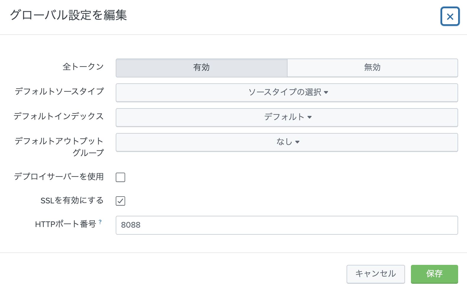
1-1. HECのGlobal設定
[設定] - [データ入力] - [HTTP Event Collector] と進みます。
右上の グローバル設定をクリックします。
全トークンを有効にして、HTTPポート (default 8088)を確認します。SSLは有効が推奨ですが、証明書がないとワーニングが上がります。(ワーニングを無視もできますが)
1-2. Token作成
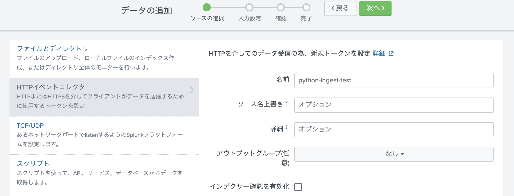
次に、Token作成をします。 一つ前の画面で右上の「新規トークン」をクリックします。
Tokenの名前を入力します。(あとはそのままでOK)
次に進んで、保存するIndexを指定します。ソースタイプは json形式になるので「自動」のままで大丈夫です。
必要に応じてIndexを新規作成して選択します。(既存のインデックスでも問題ありません)
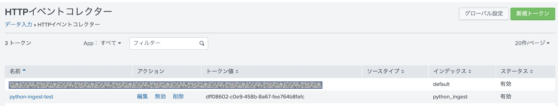
1-3. Tokenの確認
HTTP イベントコレクターの画面に戻ると、作成したトークンが確認できます。このトークンを後ほど利用します。
2. curl を使ったデータ取り込みテスト
次に RestAPIでデータが取り込めるか curlを使ってチェックします。
以下のドキュメントにサンプルがあるので、そちらを参考に実行してみます。, を変更ください。
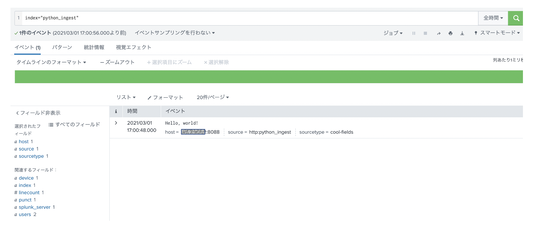
curl -k "https://<Splunk-server>:8088/services/collector/event" \
    -H "Authorization: Splunk <TOKEN>" \
    -d '{"event": "Hello, world!", "sourcetype": "cool-fields", "fields": {"device": "macbook", "users": ["joe", "bob"]}}'
無事にデータを取り込めてますね。
3. pythonでの実装
curlでできることは、pythonでも行けるので、実装は簡単なのですが、シングルイベントではなく、複数イベントを取り込む必要があるので、そのあたりを実装する必要があります。
今回は、データフレーム形式のデータを、Splunkに取り込むまでを実装したいと思います。
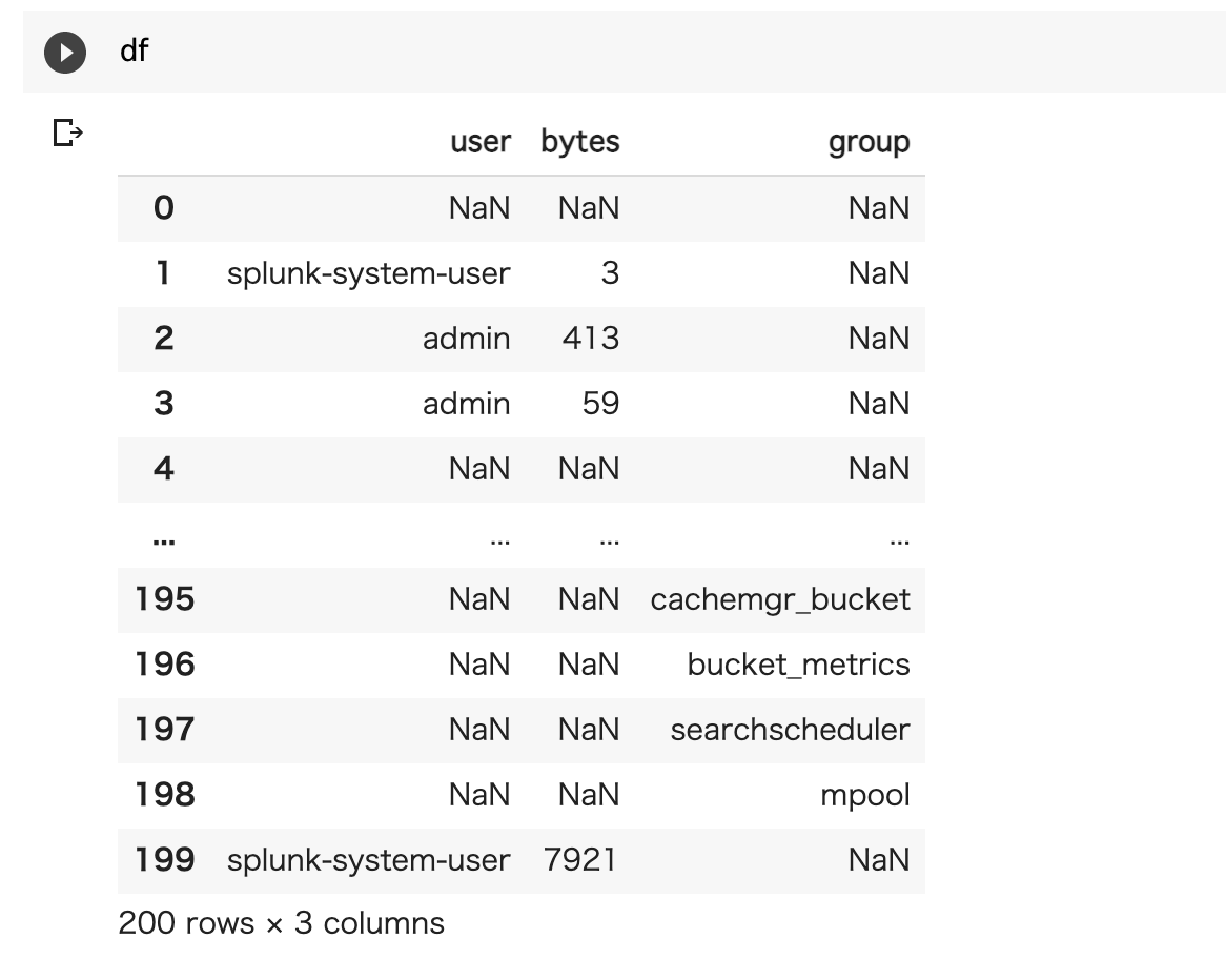
元のサンプルデータはこんな感じ(NULLが多いなー)
SpunkにHECで入れるためには、 rawデータもしくは、jsonフォーマットである必要があります。今回はjsonとして取り込もうと思います。
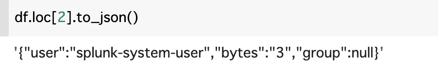
その場合、to_json()を使うことでjsonに変換できます。
これを for文を使って200件変換したデータをSplunkに取り込みたいと思います。
curlのコマンドを pythonで変換して、先ほどのデータをjsonに変換したものをループでHECに飛ばしてます。今回は証明書をセットしていないので、verify=f としてるので、ワーニングが出ますが今回は無視します。下のコードのうち、<TOKEN値>と<Server> を変更ください。
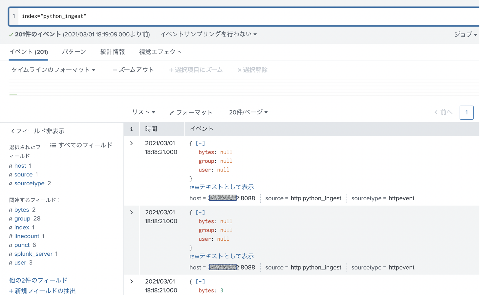
# HEC を使ったデータ投入
# Splunk Cloudの場合 443 ポートになります。

TOKEN = "<TOKEN value>"

import requests

headers = {
    'Authorization': 'Splunk ' + TOKEN,
}

for i in range(len(df.index)):

  data = '{"event": ' + df.loc[i].to_json() + '}'
  response = requests.post('https://<server>:8088/services/collector' , headers=headers, data=data, verify=False)
実行結果はこちらです。先ほどcurlコマンドでテストしたデータもあるので、全部で201件あります。json形式なのでそのままパースされてフィールド抽出まで完了してます。
最後に
大量のデータの場合、このループの方法だと時間がかかりそうなのでバッチ方式を検討した方が良さそうですが、分析で利用するためにsplunkから抜き出して、その結果をまたsplunkにフィードバックするだけなら、この方法で十分利用できそうです。
いちいちファイルに書き込んで、アップロードして。という手間が省けていい感じ。


- 投稿日:2021-03-01T18:07:17+09:00
YouTube, Deepspeech, with Google Colaboratory [testing_0005] : DeepSpeech output ’json’ [0002]
deepSpeech の音認識結果を json で受け取ると、
                                         transcripts
0  {'confidence': -1793.291259765625, 'words': [{'wor...
1  {'confidence': -87105.90625, 'words': [{'word'...
2  {'confidence': -87105.90625, 'words': [{'word'...
こうなっていました。
これは、
import pandas as pd
import json
import pprint
#from collections import OrderedDict

with open ('/content/json (1).txt','r') as f:
    #jso = json.load(f, object_pairs_hook=OrderedDict)
    line = f.read()
    #jso = json.load(f)
    jso = pd.read_json(line)
    #print(jso)
    #jso = json.loads(line)

    pprint.pprint(jso)
の結果ですが、 json をパースする方法は色々あるようですが、詳細に内容を見る前にどうなっているのかなーと開いてみるにはこの pandas で見るのが良さそうでした。
全部観ると、単語ごとの出現箇所のタイムと、尺のラップされたものになるので非常に長い行数、または一行でずー―――と続く文字列となります。
{'transcripts': [{'confidence': -1793.291259765625, 'words': [{'word': 'you', 'start_time': 0.56, 'duration': 0.12}, {'word': 'may', 'start_time': 0.74, 'duration': 0.14}, {'word': 'write', 'start_time': 1.0, 'duration': 0.2}, {'word': 'me', 'start_time': 1.3, 'duration': 0.16}, {'word': 'down', 'start_time': 1.54, 'duration': 0.18}, {'word': 'in', 'start_time': 1.84, 'duration': 0.1}, {'word': 'history', 'start_time': 2.0, 'duration': 1.06}, {'word': 'with', 'start_time': 3.12, 'duration': 0.12}, {'word': 'your', 'start_time': 3.26, 'duration': 0.16}, {'word': 'visit', 'start_time': 3.5, 'duration': 0.32}, {'word': 'wished', 'start_time': 3.86, 'duration': 0.38}, {'word': 'lines', 'start_time': 4.34, 'duration': 1.1}, {'word': 'you', 'start_time': 5.52, 'duration': 0.1}, {'word': 'may', 'start_time': 5.66, 'duration': 0.22}, {'word': 'try', 'start_time': 6.0, 'duration': 0.3}, {'word': 'me', 'start_time': 6.34, 'duration': 0.12}, {'word': 'in', 'start_time': 6.54, 'duration': 0.06}, {'word': 'the', 'start_time': 6.64, 'duration': 0.08}, {'word': 'very', 'start_time': 6.78, 'duration': 0.28}, {'word': 'dirt', 'start_time': 7.14, 'duration': 1.12}, {'word': 'but', 'start_time': 8.32, 'duration': 0.22}, {'word': 'still', 'start_time': 8.6, 'duration': 0.3}, {'word': 'like', 'start_time': 8.98, 'duration': 0.38}, {'word': 'dust', 'start_time': 9.48, 'duration': 1.48}, {'word': 'or', 'start_time': 11.1, 'duration': 1.68}, {'word': 'does', 'start_time': 12.86, 'duration': 0.24}, {'word': 'my', 'start_time': 13.16, 'duration': 0.24}, {'word': 'sauciness', 'start_time': 13.48, 'duration': 0.52}, {'word': 'upset', 'start_time': 14.06, 'duration': 0.38}, {'word': 'you', 'start_time': 14.46, 'duration': 0.72}, {'word': 'why', 'start_time': 15.36, 'duration': 0.14}, {'word': 'are', 'start_time': 15.64, 'duration': 0.12}, {'word': 'you', 'start_time': 15.8, 'duration': 0.12}, {'word': 'beside', 'start_time': 16.02, 'duration': 0.32}, {'word': 'with', 'start_time': 16.38, 'duration': 0.12}, {'word': 'gloom', 'start_time': 16.58, 'duration': 0.72}, {'word': 'to', 'start_time': 17.42, 'duration': 0.1}, {'word': 'cause', 'start_time': 17.58, 'duration': 0.22}, {'word': 'i', 'start_time': 17.88, 'duration': 0.54}, {'word': 'walk', 'start_time': 18.5, 'duration': 0.22}, {'word': 'in', 'start_time': 18.8, 'duration': 0.1}, {'word': 'the', 'start_time': 18.96, 'duration': 0.18}, {'word': 'i', 'start_time': 19.28, 'duration': 0.14}, {'word': 'have', 'start_time': 19.48, 'duration': 0.52}, {'word': 'oil', 'start_time': 20.18, 'duration': 0.38}, {'word': 'wells', 'start_time': 20.68, 'duration': 0.38}, {'word': 'pumping', 'start_time': 21.12, 'duration': 0.64}, {'word': 'my', 'start_time': 21.82, 'duration': 0.26}, {'word': 'living', 'start_time': 22.14, 'duration': 0.42}, {'word': 'room', 'start_time': 22.66, 'duration': 1.68}, {'word': 'sailors', 'start_time': 24.44, 'duration': 1.38}, {'word': 'and', 'start_time': 25.94, 'duration': 0.1}, {'word': 'like', 'start_time': 26.12, 'duration': 0.5}, {'word': 'songs', 'start_time': 26.72, 'duration': 0.32}, {'word': 'with', 'start_time': 27.1, 'duration': 0.2}, {'word': 'a', 'start_time': 27.44, 'duration': 0.1}, {'word': 'cuttenclips', 'start_time': 27.62, 'duration': 3.38}, {'word': 'springing', 'start_time': 31.02, 'duration': 0.48}, {'word': 'high', 'start_time': 31.66, 'duration': 1.2}, {'word': 'still', 'start_time': 32.92, 'duration': 0.2}, {'word': 'i', 'start_time': 33.24, 'duration': 0.14}, {'word': 'wore', 'start_time': 33.46, 'duration': 0.9}, {'word': 'did', 'start_time': 34.42, 'duration': 0.16}, {'word': 'you', 'start_time': 34.62, 'duration': 0.12}, {'word': 'want', 'start_time': 34.8, 'duration': 0.18}, {'word': 'to', 'start_time': 35.04, 'duration': 0.08}, {'word': 'see', 'start_time': 35.18, 'duration': 0.16}, {'word': 'me', 'start_time': 35.4, 'duration': 0.18}, {'word': 'broken', 'start_time': 35.64, 'duration': 1.2}, {'word': 'bowed', 'start_time': 37.0, 'duration': 0.4}, {'word': 'head', 'start_time': 37.5, 'duration': 0.22}, {'word': 'and', 'start_time': 37.82, 'duration': 0.14}, {'word': 'lord', 'start_time': 38.08, 'duration': 0.46}, {'word': 'eyes', 'start_time': 38.82, 'duration': 0.82}, {'word': 'soltali', 'start_time': 39.7, 'duration': 1.0}, {'word': 'down', 'start_time': 40.76, 'duration': 0.24}, {'word': 'like', 'start_time': 41.04, 'duration': 0.36}, {'word': 'pedrosan', 'start_time': 41.46, 'duration': 1.9}, {'word': 'by', 'start_time': 43.46, 'duration': 0.18}, {'word': 'my', 'start_time': 43.78, 'duration': 0.3}, {'word': 'soul', 'start_time': 44.18, 'duration': 0.3}, {'word': 'societaires', 'start_time': 44.5, 'duration': 2.74}, {'word': 'oudenard', 'start_time': 47.32, 'duration': 4.08}, {'word': 'isolated', 'start_time': 51.5, 'duration': 1.7}, {'word': 'as', 'start_time': 53.32, 'duration': 0.1}, {'word': 'if', 'start_time': 53.54, 'duration': 0.16}, {'word': 'i', 'start_time': 53.8, 'duration': 0.12}, {'word': 'have', 'start_time': 53.98, 'duration': 0.26}, {'word': 'gold', 'start_time': 54.36, 'duration': 0.46}, {'word': "man's", 'start_time': 54.98, 'duration': 0.36}, {'word': 'digging', 'start_time': 55.42, 'duration': 0.28}, {'word': 'in', 'start_time': 55.78, 'duration': 0.08}, {'word': 'my', 'start_time': 55.92, 'duration': 0.2}, {'word': 'own', 'start_time': 56.3, 'duration': 0.26}, {'word': 'back', 'start_time': 56.64, 'duration': 0.28}, {'word': 'yard', 'start_time': 57.0, 'duration': 1.12}, {'word': 'you', 'start_time': 58.16, 'duration': 0.12}, {'word': 'can', 'start_time': 58.34, 'duration': 0.16}, {'word': 'shoot', 'start_time': 58.54, 'duration': 0.24}, {'word': 'me', 'start_time': 58.82, 'duration': 0.14}, {'word': 'with', 'start_time': 59.0, 'duration': 0.16}, {'word': 'your', 'start_time': 59.22, 'duration': 0.18}, {'word': 'words', 'start_time': 59.54, 'duration': 0.76}, {'word': 'you', 'start_time': 60.36, 'duration': 0.14}, {'word': 'can', 'start_time': 60.56, 'duration': 0.2}, {'word': 'cut', 'start_time': 60.84, 'duration': 0.2}, {'word': 'me', 'start_time': 61.06, 'duration': 0.14}, {'word': 'with', 'start_time': 61.26, 'duration': 0.16}, {'word': 'your', 'start_time': 61.46, 'duration': 0.22}, {'word': 'lies', 'start_time': 61.84, 'duration': 0.76}, {'word': 'you', 'start_time': 62.66, 'duration': 0.14}, {'word': 'can', 'start_time': 62.86, 'duration': 0.28}, {'word': 'kill', 'start_time': 63.2, 'duration': 0.22}, {'word': 'me', 'start_time': 63.46, 'duration': 0.14}, {'word': 'with', 'start_time': 63.66, 'duration': 0.12}, {'word': 'your', 'start_time': 63.84, 'duration': 0.16}, {'word': 'hatefulness', 'start_time': 64.06, 'duration': 0.54}, {'word': 'but', 'start_time': 64.66, 'duration': 0.1}, {'word': 'just', 'start_time': 64.84, 'duration': 0.26}, {'word': 'like', 'start_time': 65.14, 'duration': 0.42}, {'word': 'life', 'start_time': 65.64, 'duration': 1.42}, {'word': 'i', 'start_time': 67.18, 'duration': 1.46}, {'word': 'does', 'start_time': 68.68, 'duration': 0.24}, {'word': 'my', 'start_time': 68.96, 'duration': 0.26}, {'word': 'senatorian', 'start_time': 69.28, 'duration': 12.02}, {'word': 'as', 'start_time': 81.4, 'duration': 0.18}, {'word': 'if', 'start_time': 81.72, 'duration': 0.22}, {'word': 'i', 'start_time': 82.06, 'duration': 0.1}, {'word': 'have', 'start_time': 82.22, 'duration': 0.26}, {'word': 'diamonds', 'start_time': 82.56, 'duration': 0.5}, {'word': 'at', 'start_time': 83.16, 'duration': 0.1}, {'word': 'the', 'start_time': 83.3, 'duration': 0.1}, {'word': 'meeting', 'start_time': 83.46, 'duration': 0.4}, {'word': 'of', 'start_time': 84.0, 'duration': 0.12}, {'word': 'my', 'start_time': 84.22, 'duration': 0.3}, {'word': 'time', 'start_time': 84.72, 'duration': 2.72}, {'word': 'out', 'start_time': 87.58, 'duration': 0.18}, {'word': 'of', 'start_time': 87.84, 'duration': 0.12}, {'word': 'the', 'start_time': 88.0, 'duration': 0.12}, {'word': 'huts', 'start_time': 88.18, 'duration': 0.28}, {'word': 'of', 'start_time': 88.56, 'duration': 0.12}, {'word': 'history', 'start_time': 88.76, 'duration': 0.74}, {'word': 'shame', 'start_time': 89.6, 'duration': 0.32}, {'word': 'i', 'start_time': 90.04, 'duration': 0.18}, {'word': 'rise', 'start_time': 90.38, 'duration': 1.2}, {'word': 'up', 'start_time': 91.7, 'duration': 0.1}, {'word': 'from', 'start_time': 91.84, 'duration': 0.16}, {'word': 'a', 'start_time': 92.14, 'duration': 0.08}, {'word': 'past', 'start_time': 92.28, 'duration': 0.34}, {'word': 'rooted', 'start_time': 92.7, 'duration': 0.36}, {'word': 'in', 'start_time': 93.18, 'duration': 0.18}, {'word': 'pain', 'start_time': 93.46, 'duration': 0.72}, {'word': 'i', 'start_time': 94.32, 'duration': 0.14}, {'word': 'ran', 'start_time': 94.54, 'duration': 0.94}, {'word': 'a', 'start_time': 95.62, 'duration': 0.06}, {'word': 'black', 'start_time': 95.72, 'duration': 0.26}, {'word': 'ocean', 'start_time': 96.06, 'duration': 0.56}, {'word': 'heaving', 'start_time': 96.74, 'duration': 0.44}, {'word': 'and', 'start_time': 97.28, 'duration': 0.22}, {'word': 'would', 'start_time': 97.74, 'duration': 0.92}, {'word': 'willingly', 'start_time': 98.76, 'duration': 1.32}, {'word': 'and', 'start_time': 100.22, 'duration': 0.14}, {'word': 'bearing', 'start_time': 100.44, 'duration': 0.3}, {'word': 'it', 'start_time': 100.82, 'duration': 1.8}, {'word': 'leaving', 'start_time': 102.66, 'duration': 0.36}, {'word': 'behind', 'start_time': 103.1, 'duration': 0.56}, {'word': 'it', 'start_time': 103.78, 'duration': 0.2}, {'word': 'of', 'start_time': 104.1, 'duration': 0.14}, {'word': 'terror', 'start_time': 104.32, 'duration': 0.64}, {'word': 'and', 'start_time': 105.1, 'duration': 0.32}, {'word': 'fear', 'start_time': 105.54, 'duration': 0.8}, {'word': 'as', 'start_time': 107.04, 'duration': 0.9}, {'word': 'into', 'start_time': 108.14, 'duration': 0.3}, {'word': 'a', 'start_time': 108.52, 'duration': 0.06}, {'word': 'daybreak', 'start_time': 108.64, 'duration': 0.54}, {'word': 'miraculously', 'start_time': 109.24, 'duration': 1.04}, {'word': 'clear', 'start_time': 110.34, 'duration': 1.26}, {'word': 'in', 'start_time': 111.74, 'duration': 1.42}, {'word': 'bringing', 'start_time': 113.22, 'duration': 0.42}, {'word': 'the', 'start_time': 113.7, 'duration': 0.1}, {'word': 'gifts', 'start_time': 113.86, 'duration': 0.32}, {'word': 'that', 'start_time': 114.24, 'duration': 0.22}, {'word': 'my', 'start_time': 114.56, 'duration': 0.18}, {'word': 'ancestors', 'start_time': 114.86, 'duration': 0.66}, {'word': 'gave', 'start_time': 115.66, 'duration': 0.8}, {'word': 'i', 'start_time': 116.64, 'duration': 0.12}, {'word': 'am', 'start_time': 116.84, 'duration': 0.14}, {'word': 'the', 'start_time': 117.06, 'duration': 0.24}, {'word': 'whole', 'start_time': 117.4, 'duration': 0.58}, {'word': 'and', 'start_time': 118.1, 'duration': 0.1}, {'word': 'the', 'start_time': 118.26, 'duration': 0.18}, {'word': 'dream', 'start_time': 118.54, 'duration': 0.78}, {'word': 'of', 'start_time': 119.38, 'duration': 0.1}, {'word': 'the', 'start_time': 119.54, 'duration': 0.22}, {'word': 'slave', 'start_time': 119.8, 'duration': 1.18}, {'word': 'and', 'start_time': 121.2, 'duration': 0.3}, {'word': 'so', 'start_time': 121.64, 'duration': 4.68}, {'word': 'that', 'start_time': 126.42, 'duration': 0.14}]}, {'confidence': -1795.8509521484375, 'words': [{'word': 'you', 'start_time': 0.56, 'duration': 0.12}, {'word': 'may', 'start_time': 0.74, 'duration': 0.14}, {'word': 'write', 'start_time': 1.0, 'duration': 0.2}, {'word': 'me', 'start_time': 1.3, 'duration': 0.16}, {'word': 'down', 'start_time': 1.54, 'duration': 0.18}, {'word': 'in', 'start_time': 1.84, 'duration': 0.1}, {'word': 'history', 'start_time': 2.0, 'duration': 1.06}, {'word': 'with', 'start_time': 3.12, 'duration': 0.12}, {'word': 'your', 'start_time': 3.26, 'duration': 0.16}, {'word': 'visit', 'start_time': 3.5, 'duration': 0.32}, {'word': 'wished', 'start_time': 3.86, 'duration': 0.38}, {'word': 'lines', 'start_time': 4.34, 'duration': 1.1}, {'word': 'you', 'start_time': 5.52, 'duration': 0.1}, {'word': 'may', 'start_time': 5.66, 'duration': 0.22}, {'word': 'try', 'start_time': 6.0, 'duration': 0.3}, {'word': 'me', 'start_time': 6.34, 'duration': 0.12}, {'word': 'in', 'start_time': 6.54, 'duration': 0.06}, {'word': 'the', 'start_time': 6.64, 'duration': 0.08}, {'word': 'very', 'start_time': 6.78, 'duration': 0.28}, {'word': 'dirt', 'start_time': 7.14, 'duration': 1.12}, {'word': 'but', 'start_time': 8.32, 'duration': 0.22}, {'word': 'still', 'start_time': 8.6, 'duration': 0.3}, {'word': 'like', 'start_time': 8.98, 'duration': 0.38}, {'word': 'dust', 'start_time': 9.48, 'duration': 1.48}, {'word': 'or', 'start_time': 11.1, 'duration': 1.68}, {'word': 'does', 'start_time': 12.86, 'duration': 0.24}, {'word': 'my', 'start_time': 13.16, 'duration': 0.24}, {'word': 'sauciness', 'start_time': 13.48, 'duration': 0.52}, {'word': 'upset', 'start_time': 14.06, 'duration': 0.38}, {'word': 'you', 'start_time': 14.46, 'duration': 0.72}, {'word': 'why', 'start_time': 15.36, 'duration': 0.14}, {'word': 'are', 'start_time': 15.64, 'duration': 0.12}, {'word': 'you', 'start_time': 15.8, 'duration': 0.12}, {'word': 'beside', 'start_time': 16.02, 'duration': 0.32}, {'word': 'with', 'start_time': 16.38, 'duration': 0.12}, {'word': 'gloom', 'start_time': 16.58, 'duration': 0.72}, {'word': 'to', 'start_time': 17.42, 'duration': 0.1}, {'word': 'cause', 'start_time': 17.58, 'duration': 0.22}, {'word': 'i', 'start_time': 17.88, 'duration': 0.54}, {'word': 'walk', 'start_time': 18.5, 'duration': 0.22}, {'word': 'in', 'start_time': 18.8, 'duration': 0.1}, {'word': 'the', 'start_time': 18.96, 'duration': 0.18}, {'word': 'i', 'start_time': 19.28, 'duration': 0.14}, {'word': 'have', 'start_time': 19.48, 'duration': 0.52}, {'word': 'oil', 'start_time': 20.18, 'duration': 0.38}, {'word': 'wells', 'start_time': 20.68, 'duration': 0.38}, {'word': 'pumping', 'start_time': 21.12, 'duration': 0.64}, {'word': 'my', 'start_time': 21.82, 'duration': 0.26}, {'word': 'living', 'start_time': 22.14, 'duration': 0.42}, {'word': 'room', 'start_time': 22.66, 'duration': 1.68}, {'word': 'sailors', 'start_time': 24.44, 'duration': 1.38}, {'word': 'and', 'start_time': 25.94, 'duration': 0.1}, {'word': 'like', 'start_time': 26.12, 'duration': 0.5}, {'word': 'songs', 'start_time': 26.72, 'duration': 0.32}, {'word': 'with', 'start_time': 27.1, 'duration': 0.2}, {'word': 'a', 'start_time': 27.44, 'duration': 0.1}, {'word': 'cuttenclips', 'start_time': 27.62, 'duration': 3.38}, {'word': 'springing', 'start_time': 31.02, 'duration': 0.48}, {'word': 'high', 'start_time': 31.66, 'duration': 1.2}, {'word': 'still', 'start_time': 32.92, 'duration': 0.2}, {'word': 'i', 'start_time': 33.24, 'duration': 0.14}, {'word': 'wore', 'start_time': 33.46, 'duration': 0.9}, {'word': 'did', 'start_time': 34.42, 'duration': 0.16}, {'word': 'you', 'start_time': 34.62, 'duration': 0.12}, {'word': 'want', 'start_time': 34.8, 'duration': 0.18}, {'word': 'to', 'start_time': 35.04, 'duration': 0.08}, {'word': 'see', 'start_time': 35.18, 'duration': 0.16}, {'word': 'me', 'start_time': 35.4, 'duration': 0.18}, {'word': 'broken', 'start_time': 35.64, 'duration': 1.2}, {'word': 'bowed', 'start_time': 37.0, 'duration': 0.4}, {'word': 'head', 'start_time': 37.5, 'duration': 0.22}, {'word': 'and', 'start_time': 37.82, 'duration': 0.14}, {'word': 'lord', 'start_time': 38.08, 'duration': 0.46}, {'word': 'eyes', 'start_time': 38.82, 'duration': 0.82}, {'word': 'soltali', 'start_time': 39.7, 'duration': 1.0}, {'word': 'down', 'start_time': 40.76, 'duration': 0.24}, {'word': 'like', 'start_time': 41.04, 'duration': 0.36}, {'word': 'pedrosan', 'start_time': 41.46, 'duration': 1.9}, {'word': 'by', 'start_time': 43.46, 'duration': 0.18}, {'word': 'my', 'start_time': 43.78, 'duration': 0.3}, {'word': 'soul', 'start_time': 44.18, 'duration': 0.3}, {'word': 'societaires', 'start_time': 44.5, 'duration': 2.74}, {'word': 'oudenard', 'start_time': 47.32, 'duration': 4.08}, {'word': 'isolated', 'start_time': 51.5, 'duration': 1.7}, {'word': 'as', 'start_time': 53.32, 'duration': 0.1}, {'word': 'if', 'start_time': 53.54, 'duration': 0.16}, {'word': 'i', 'start_time': 53.8, 'duration': 0.12}, {'word': 'have', 'start_time': 53.98, 'duration': 0.26}, {'word': 'gold', 'start_time': 54.36, 'duration': 0.46}, {'word': "man's", 'start_time': 54.98, 'duration': 0.36}, {'word': 'digging', 'start_time': 55.42, 'duration': 0.28}, {'word': 'in', 'start_time': 55.78, 'duration': 0.08}, {'word': 'my', 'start_time': 55.92, 'duration': 0.2}, {'word': 'own', 'start_time': 56.3, 'duration': 0.26}, {'word': 'back', 'start_time': 56.64, 'duration': 0.28}, {'word': 'yard', 'start_time': 57.0, 'duration': 1.12}, {'word': 'you', 'start_time': 58.16, 'duration': 0.12}, {'word': 'can', 'start_time': 58.34, 'duration': 0.16}, {'word': 'shoot', 'start_time': 58.54, 'duration': 0.24}, {'word': 'me', 'start_time': 58.82, 'duration': 0.14}, {'word': 'with', 'start_time': 59.0, 'duration': 0.16}, {'word': 'your', 'start_time': 59.22, 'duration': 0.18}, {'word': 'words', 'start_time': 59.54, 'duration': 0.76}, {'word': 'you', 'start_time': 60.36, 'duration': 0.14}, {'word': 'can', 'start_time': 60.56, 'duration': 0.2}, {'word': 'cut', 'start_time': 60.84, 'duration': 0.2}, {'word': 'me', 'start_time': 61.06, 'duration': 0.14}, {'word': 'with', 'start_time': 61.26, 'duration': 0.16}, {'word': 'your', 'start_time': 61.46, 'duration': 0.22}, {'word': 'lies', 'start_time': 61.84, 'duration': 0.76}, {'word': 'you', 'start_time': 62.66, 'duration': 0.14}, {'word': 'can', 'start_time': 62.86, 'duration': 0.28}, {'word': 'kill', 'start_time': 63.2, 'duration': 0.22}, {'word': 'me', 'start_time': 63.46, 'duration': 0.14}, {'word': 'with', 'start_time': 63.66, 'duration': 0.12}, {'word': 'your', 'start_time': 63.84, 'duration': 0.16}, {'word': 'hatefulness', 'start_time': 64.06, 'duration': 0.54}, {'word': 'but', 'start_time': 64.66, 'duration': 0.1}, {'word': 'just', 'start_time': 64.84, 'duration': 0.26}, {'word': 'like', 'start_time': 65.14, 'duration': 0.42}, {'word': 'life', 'start_time': 65.64, 'duration': 1.42}, {'word': 'i', 'start_time': 67.18, 'duration': 1.46}, {'word': 'does', 'start_time': 68.68, 'duration': 0.24}, {'word': 'my', 'start_time': 68.96, 'duration': 0.26}, {'word': 'senatorian', 'start_time': 69.28, 'duration': 12.02}, {'word': 'as', 'start_time': 81.4, 'duration': 0.18}, {'word': 'if', 'start_time': 81.72, 'duration': 0.22}, {'word': 'i', 'start_time': 82.06, 'duration': 0.1}, {'word': 'have', 'start_time': 82.22, 'duration': 0.26}, {'word': 'diamonds', 'start_time': 82.56, 'duration': 0.5}, {'word': 'at', 'start_time': 83.16, 'duration': 0.1}, {'word': 'the', 'start_time': 83.3, 'duration': 0.1}, {'word': 'meeting', 'start_time': 83.46, 'duration': 0.4}, {'word': 'of', 'start_time': 84.0, 'duration': 0.12}, {'word': 'my', 'start_time': 84.22, 'duration': 0.3}, {'word': 'time', 'start_time': 84.72, 'duration': 2.72}, {'word': 'out', 'start_time': 87.58, 'duration': 0.18}, {'word': 'of', 'start_time': 87.84, 'duration': 0.12}, {'word': 'the', 'start_time': 88.0, 'duration': 0.12}, {'word': 'huts', 'start_time': 88.18, 'duration': 0.28}, {'word': 'of', 'start_time': 88.56, 'duration': 0.12}, {'word': 'history', 'start_time': 88.76, 'duration': 0.74}, {'word': 'shame', 'start_time': 89.6, 'duration': 0.32}, {'word': 'i', 'start_time': 90.04, 'duration': 0.18}, {'word': 'rise', 'start_time': 90.38, 'duration': 1.2}, {'word': 'up', 'start_time': 91.7, 'duration': 0.1}, {'word': 'from', 'start_time': 91.84, 'duration': 0.16}, {'word': 'a', 'start_time': 92.14, 'duration': 0.08}, {'word': 'past', 'start_time': 92.28, 'duration': 0.34}, {'word': 'rooted', 'start_time': 92.7, 'duration': 0.36}, {'word': 'in', 'start_time': 93.18, 'duration': 0.18}, {'word': 'pain', 'start_time': 93.46, 'duration': 0.72}, {'word': 'i', 'start_time': 94.32, 'duration': 0.14}, {'word': 'ran', 'start_time': 94.54, 'duration': 0.94}, {'word': 'a', 'start_time': 95.62, 'duration': 0.06}, {'word': 'black', 'start_time': 95.72, 'duration': 0.26}, {'word': 'ocean', 'start_time': 96.06, 'duration': 0.56}, {'word': 'heaving', 'start_time': 96.74, 'duration': 0.44}, {'word': 'and', 'start_time': 97.28, 'duration': 0.22}, {'word': 'would', 'start_time': 97.74, 'duration': 0.92}, {'word': 'willingly', 'start_time': 98.76, 'duration': 1.32}, {'word': 'and', 'start_time': 100.22, 'duration': 0.14}, {'word': 'bearing', 'start_time': 100.44, 'duration': 0.3}, {'word': 'it', 'start_time': 100.82, 'duration': 1.8}, {'word': 'leaving', 'start_time': 102.66, 'duration': 0.36}, {'word': 'behind', 'start_time': 103.1, 'duration': 0.56}, {'word': 'it', 'start_time': 103.78, 'duration': 0.2}, {'word': 'of', 'start_time': 104.1, 'duration': 0.14}, {'word': 'terror', 'start_time': 104.32, 'duration': 0.64}, {'word': 'and', 'start_time': 105.1, 'duration': 0.32}, {'word': 'fear', 'start_time': 105.54, 'duration': 0.8}, {'word': 'as', 'start_time': 107.04, 'duration': 0.9}, {'word': 'into', 'start_time': 108.14, 'duration': 0.3}, {'word': 'a', 'start_time': 108.52, 'duration': 0.06}, {'word': 'daybreak', 'start_time': 108.64, 'duration': 0.54}, {'word': 'miraculously', 'start_time': 109.24, 'duration': 1.04}, {'word': 'clear', 'start_time': 110.34, 'duration': 1.26}, {'word': 'in', 'start_time': 111.74, 'duration': 1.42}, {'word': 'bringing', 'start_time': 113.22, 'duration': 0.42}, {'word': 'the', 'start_time': 113.7, 'duration': 0.1}, {'word': 'gifts', 'start_time': 113.86, 'duration': 0.32}, {'word': 'that', 'start_time': 114.24, 'duration': 0.22}, {'word': 'my', 'start_time': 114.56, 'duration': 0.18}, {'word': 'ancestors', 'start_time': 114.86, 'duration': 0.66}, {'word': 'gave', 'start_time': 115.66, 'duration': 0.8}, {'word': 'i', 'start_time': 116.64, 'duration': 0.12}, {'word': 'am', 'start_time': 116.84, 'duration': 0.14}, {'word': 'the', 'start_time': 117.06, 'duration': 0.24}, {'word': 'whole', 'start_time': 117.4, 'duration': 0.58}, {'word': 'and', 'start_time': 118.1, 'duration': 0.1}, {'word': 'the', 'start_time': 118.26, 'duration': 0.18}, {'word': 'dream', 'start_time': 118.54, 'duration': 0.78}, {'word': 'of', 'start_time': 119.38, 'duration': 0.1}, {'word': 'the', 'start_time': 119.54, 'duration': 0.22}, {'word': 'slave', 'start_time': 119.8, 'duration': 1.18}, {'word': 'and', 'start_time': 121.2, 'duration': 0.3}, {'word': 'so', 'start_time': 121.64, 'duration': 4.68}, {'word': 'then', 'start_time': 126.42, 'duration': 0.14}]}, {'confidence': -1796.1273193359375, 'words': [{'word': 'you', 'start_time': 0.56, 'duration': 0.12}, {'word': 'may', 'start_time': 0.74, 'duration': 0.14}, {'word': 'write', 'start_time': 1.0, 'duration': 0.2}, {'word': 'me', 'start_time': 1.3, 'duration': 0.16}, {'word': 'down', 'start_time': 1.54, 'duration': 0.18}, {'word': 'in', 'start_time': 1.84, 'duration': 0.1}, {'word': 'history', 'start_time': 2.0, 'duration': 1.06}, {'word': 'with', 'start_time': 3.12, 'duration': 0.12}, {'word': 'your', 'start_time': 3.26, 'duration': 0.16}, {'word': 'visit', 'start_time': 3.5, 'duration': 0.32}, {'word': 'wished', 'start_time': 3.86, 'duration': 0.38}, {'word': 'lines', 'start_time': 4.34, 'duration': 1.1}, {'word': 'you', 'start_time': 5.52, 'duration': 0.1}, {'word': 'may', 'start_time': 5.66, 'duration': 0.22}, {'word': 'try', 'start_time': 6.0, 'duration': 0.3}, {'word': 'me', 'start_time': 6.34, 'duration': 0.12}, {'word': 'in', 'start_time': 6.54, 'duration': 0.06}, {'word': 'the', 'start_time': 6.64, 'duration': 0.08}, {'word': 'very', 'start_time': 6.78, 'duration': 0.28}, {'word': 'dirt', 'start_time': 7.14, 'duration': 1.12}, {'word': 'but', 'start_time': 8.32, 'duration': 0.22}, {'word': 'still', 'start_time': 8.6, 'duration': 0.3}, {'word': 'like', 'start_time': 8.98, 'duration': 0.38}, {'word': 'dust', 'start_time': 9.48, 'duration': 1.48}, {'word': 'or', 'start_time': 11.1, 'duration': 1.68}, {'word': 'does', 'start_time': 12.86, 'duration': 0.24}, {'word': 'my', 'start_time': 13.16, 'duration': 0.24}, {'word': 'sauciness', 'start_time': 13.48, 'duration': 0.52}, {'word': 'upset', 'start_time': 14.06, 'duration': 0.38}, {'word': 'you', 'start_time': 14.46, 'duration': 0.72}, {'word': 'why', 'start_time': 15.36, 'duration': 0.14}, {'word': 'are', 'start_time': 15.64, 'duration': 0.12}, {'word': 'you', 'start_time': 15.8, 'duration': 0.12}, {'word': 'beside', 'start_time': 16.02, 'duration': 0.32}, {'word': 'with', 'start_time': 16.38, 'duration': 0.12}, {'word': 'gloom', 'start_time': 16.58, 'duration': 0.72}, {'word': 'to', 'start_time': 17.42, 'duration': 0.1}, {'word': 'cause', 'start_time': 17.58, 'duration': 0.22}, {'word': 'i', 'start_time': 17.88, 'duration': 0.54}, {'word': 'walk', 'start_time': 18.5, 'duration': 0.22}, {'word': 'in', 'start_time': 18.8, 'duration': 0.1}, {'word': 'the', 'start_time': 18.96, 'duration': 0.18}, {'word': 'i', 'start_time': 19.28, 'duration': 0.14}, {'word': 'have', 'start_time': 19.48, 'duration': 0.52}, {'word': 'oil', 'start_time': 20.18, 'duration': 0.38}, {'word': 'wells', 'start_time': 20.68, 'duration': 0.38}, {'word': 'pumping', 'start_time': 21.12, 'duration': 0.64}, {'word': 'my', 'start_time': 21.82, 'duration': 0.26}, {'word': 'living', 'start_time': 22.14, 'duration': 0.42}, {'word': 'room', 'start_time': 22.66, 'duration': 1.68}, {'word': 'sailors', 'start_time': 24.44, 'duration': 1.38}, {'word': 'and', 'start_time': 25.94, 'duration': 0.1}, {'word': 'like', 'start_time': 26.12, 'duration': 0.5}, {'word': 'songs', 'start_time': 26.72, 'duration': 0.32}, {'word': 'with', 'start_time': 27.1, 'duration': 0.2}, {'word': 'a', 'start_time': 27.44, 'duration': 0.1}, {'word': 'cuttenclips', 'start_time': 27.62, 'duration': 3.38}, {'word': 'springing', 'start_time': 31.02, 'duration': 0.48}, {'word': 'high', 'start_time': 31.66, 'duration': 1.2}, {'word': 'still', 'start_time': 32.92, 'duration': 0.2}, {'word': 'i', 'start_time': 33.24, 'duration': 0.14}, {'word': 'wore', 'start_time': 33.46, 'duration': 0.9}, {'word': 'did', 'start_time': 34.42, 'duration': 0.16}, {'word': 'you', 'start_time': 34.62, 'duration': 0.12}, {'word': 'want', 'start_time': 34.8, 'duration': 0.18}, {'word': 'to', 'start_time': 35.04, 'duration': 0.08}, {'word': 'see', 'start_time': 35.18, 'duration': 0.16}, {'word': 'me', 'start_time': 35.4, 'duration': 0.18}, {'word': 'broken', 'start_time': 35.64, 'duration': 1.2}, {'word': 'bowed', 'start_time': 37.0, 'duration': 0.4}, {'word': 'head', 'start_time': 37.5, 'duration': 0.22}, {'word': 'and', 'start_time': 37.82, 'duration': 0.14}, {'word': 'lord', 'start_time': 38.08, 'duration': 0.46}, {'word': 'eyes', 'start_time': 38.82, 'duration': 0.82}, {'word': 'soltali', 'start_time': 39.7, 'duration': 1.0}, {'word': 'down', 'start_time': 40.76, 'duration': 0.24}, {'word': 'like', 'start_time': 41.04, 'duration': 0.36}, {'word': 'pedrosan', 'start_time': 41.46, 'duration': 1.9}, {'word': 'by', 'start_time': 43.46, 'duration': 0.18}, {'word': 'my', 'start_time': 43.78, 'duration': 0.3}, {'word': 'soul', 'start_time': 44.18, 'duration': 0.3}, {'word': 'societaires', 'start_time': 44.5, 'duration': 2.74}, {'word': 'oudenard', 'start_time': 47.32, 'duration': 4.08}, {'word': 'isolated', 'start_time': 51.5, 'duration': 1.7}, {'word': 'as', 'start_time': 53.32, 'duration': 0.1}, {'word': 'if', 'start_time': 53.54, 'duration': 0.16}, {'word': 'i', 'start_time': 53.8, 'duration': 0.12}, {'word': 'have', 'start_time': 53.98, 'duration': 0.26}, {'word': 'gold', 'start_time': 54.36, 'duration': 0.46}, {'word': "man's", 'start_time': 54.98, 'duration': 0.36}, {'word': 'digging', 'start_time': 55.42, 'duration': 0.28}, {'word': 'in', 'start_time': 55.78, 'duration': 0.08}, {'word': 'my', 'start_time': 55.92, 'duration': 0.2}, {'word': 'own', 'start_time': 56.3, 'duration': 0.26}, {'word': 'back', 'start_time': 56.64, 'duration': 0.28}, {'word': 'yard', 'start_time': 57.0, 'duration': 1.12}, {'word': 'you', 'start_time': 58.16, 'duration': 0.12}, {'word': 'can', 'start_time': 58.34, 'duration': 0.16}, {'word': 'shoot', 'start_time': 58.54, 'duration': 0.24}, {'word': 'me', 'start_time': 58.82, 'duration': 0.14}, {'word': 'with', 'start_time': 59.0, 'duration': 0.16}, {'word': 'your', 'start_time': 59.22, 'duration': 0.18}, {'word': 'words', 'start_time': 59.54, 'duration': 0.76}, {'word': 'you', 'start_time': 60.36, 'duration': 0.14}, {'word': 'can', 'start_time': 60.56, 'duration': 0.2}, {'word': 'cut', 'start_time': 60.84, 'duration': 0.2}, {'word': 'me', 'start_time': 61.06, 'duration': 0.14}, {'word': 'with', 'start_time': 61.26, 'duration': 0.16}, {'word': 'your', 'start_time': 61.46, 'duration': 0.22}, {'word': 'lies', 'start_time': 61.84, 'duration': 0.76}, {'word': 'you', 'start_time': 62.66, 'duration': 0.14}, {'word': 'can', 'start_time': 62.86, 'duration': 0.28}, {'word': 'kill', 'start_time': 63.2, 'duration': 0.22}, {'word': 'me', 'start_time': 63.46, 'duration': 0.14}, {'word': 'with', 'start_time': 63.66, 'duration': 0.12}, {'word': 'your', 'start_time': 63.84, 'duration': 0.16}, {'word': 'hatefulness', 'start_time': 64.06, 'duration': 0.54}, {'word': 'but', 'start_time': 64.66, 'duration': 0.1}, {'word': 'just', 'start_time': 64.84, 'duration': 0.26}, {'word': 'like', 'start_time': 65.14, 'duration': 0.42}, {'word': 'life', 'start_time': 65.64, 'duration': 1.42}, {'word': 'i', 'start_time': 67.18, 'duration': 1.46}, {'word': 'does', 'start_time': 68.68, 'duration': 0.24}, {'word': 'my', 'start_time': 68.96, 'duration': 0.26}, {'word': 'senatorian', 'start_time': 69.28, 'duration': 12.02}, {'word': 'as', 'start_time': 81.4, 'duration': 0.18}, {'word': 'if', 'start_time': 81.72, 'duration': 0.22}, {'word': 'i', 'start_time': 82.06, 'duration': 0.1}, {'word': 'have', 'start_time': 82.22, 'duration': 0.26}, {'word': 'diamonds', 'start_time': 82.56, 'duration': 0.5}, {'word': 'at', 'start_time': 83.16, 'duration': 0.1}, {'word': 'the', 'start_time': 83.3, 'duration': 0.1}, {'word': 'meeting', 'start_time': 83.46, 'duration': 0.4}, {'word': 'of', 'start_time': 84.0, 'duration': 0.12}, {'word': 'my', 'start_time': 84.22, 'duration': 0.3}, {'word': 'time', 'start_time': 84.72, 'duration': 2.72}, {'word': 'out', 'start_time': 87.58, 'duration': 0.18}, {'word': 'of', 'start_time': 87.84, 'duration': 0.12}, {'word': 'the', 'start_time': 88.0, 'duration': 0.12}, {'word': 'huts', 'start_time': 88.18, 'duration': 0.28}, {'word': 'of', 'start_time': 88.56, 'duration': 0.12}, {'word': 'history', 'start_time': 88.76, 'duration': 0.74}, {'word': 'shame', 'start_time': 89.6, 'duration': 0.32}, {'word': 'i', 'start_time': 90.04, 'duration': 0.18}, {'word': 'rise', 'start_time': 90.38, 'duration': 1.2}, {'word': 'up', 'start_time': 91.7, 'duration': 0.1}, {'word': 'from', 'start_time': 91.84, 'duration': 0.16}, {'word': 'a', 'start_time': 92.14, 'duration': 0.08}, {'word': 'past', 'start_time': 92.28, 'duration': 0.34}, {'word': 'rooted', 'start_time': 92.7, 'duration': 0.36}, {'word': 'in', 'start_time': 93.18, 'duration': 0.18}, {'word': 'pain', 'start_time': 93.46, 'duration': 0.72}, {'word': 'i', 'start_time': 94.32, 'duration': 0.14}, {'word': 'ran', 'start_time': 94.54, 'duration': 0.94}, {'word': 'a', 'start_time': 95.62, 'duration': 0.06}, {'word': 'black', 'start_time': 95.72, 'duration': 0.26}, {'word': 'ocean', 'start_time': 96.06, 'duration': 0.56}, {'word': 'heaving', 'start_time': 96.74, 'duration': 0.44}, {'word': 'and', 'start_time': 97.28, 'duration': 0.22}, {'word': 'would', 'start_time': 97.74, 'duration': 0.92}, {'word': 'willingly', 'start_time': 98.76, 'duration': 1.32}, {'word': 'and', 'start_time': 100.22, 'duration': 0.14}, {'word': 'bearing', 'start_time': 100.44, 'duration': 0.3}, {'word': 'it', 'start_time': 100.82, 'duration': 1.8}, {'word': 'leaving', 'start_time': 102.66, 'duration': 0.36}, {'word': 'behind', 'start_time': 103.1, 'duration': 0.56}, {'word': 'it', 'start_time': 103.78, 'duration': 0.2}, {'word': 'of', 'start_time': 104.1, 'duration': 0.14}, {'word': 'terror', 'start_time': 104.32, 'duration': 0.64}, {'word': 'and', 'start_time': 105.1, 'duration': 0.32}, {'word': 'fear', 'start_time': 105.54, 'duration': 0.8}, {'word': 'as', 'start_time': 107.04, 'duration': 0.9}, {'word': 'into', 'start_time': 108.14, 'duration': 0.3}, {'word': 'a', 'start_time': 108.52, 'duration': 0.06}, {'word': 'daybreak', 'start_time': 108.64, 'duration': 0.54}, {'word': 'miraculously', 'start_time': 109.24, 'duration': 1.04}, {'word': 'clear', 'start_time': 110.34, 'duration': 1.26}, {'word': 'in', 'start_time': 111.74, 'duration': 1.42}, {'word': 'bringing', 'start_time': 113.22, 'duration': 0.42}, {'word': 'the', 'start_time': 113.7, 'duration': 0.1}, {'word': 'gifts', 'start_time': 113.86, 'duration': 0.32}, {'word': 'that', 'start_time': 114.24, 'duration': 0.22}, {'word': 'my', 'start_time': 114.56, 'duration': 0.18}, {'word': 'ancestors', 'start_time': 114.86, 'duration': 0.66}, {'word': 'gave', 'start_time': 115.66, 'duration': 0.8}, {'word': 'i', 'start_time': 116.64, 'duration': 0.12}, {'word': 'am', 'start_time': 116.84, 'duration': 0.14}, {'word': 'the', 'start_time': 117.06, 'duration': 0.24}, {'word': 'whole', 'start_time': 117.4, 'duration': 0.58}, {'word': 'and', 'start_time': 118.1, 'duration': 0.1}, {'word': 'the', 'start_time': 118.26, 'duration': 0.18}, {'word': 'dream', 'start_time': 118.54, 'duration': 0.78}, {'word': 'of', 'start_time': 119.38, 'duration': 0.1}, {'word': 'the', 'start_time': 119.54, 'duration': 0.22}, {'word': 'slaves', 'start_time': 119.8, 'duration': 1.18}, {'word': 'and', 'start_time': 121.2, 'duration': 0.3}, {'word': 'so', 'start_time': 121.64, 'duration': 4.68}, {'word': 'then', 'start_time': 126.42, 'duration': 0.14}]}]}ちょっとまだ
confidenceを理解していないのですが、きっと認識の候補かなぁ...と仮定して、['transcripts'][0]つまりtranscripts 0 {'confidence': -1793.291259765625, 'words': [{'wor...のなかのものを抽出して、json から SubRip 形式の(つまり YouTube でデフォルトで使われている字幕のファイル形式ですが)ファイルに変換する python のコードを考えてみました。GoogleColab 用ですが、別にこれはたんに json ファイル、ここではなぜか、
.jsonではなく.txtにしていますが、から json をパースするプログラムなので、ローカル用に変更して実行しても十分速いのではないかなと思います。やってないので、「(やっ)タラ、(もし、や)レバ」です。import json import datetime from google.colab import files import sys #uploaded = files.upload() upfilename = '/content/json (1).txt' #for fn in uploaded.keys(): # print('User uploaded file "{name}" with length {length} bytes'.format(name=fn, length=len(uploaded[fn]))) # upfilename = fn def fmttime(seconds): secs = seconds #millisecs / 1000.0 d = datetime.timedelta(seconds=secs) t = (datetime.datetime.min + d).time() milli = t.strftime('%f')[:3] value = t.strftime('%H:%M:%S,') + milli return value original_stdout = sys.stdout #""" stdout backup """ filename = 'subtitle.srt' #""" print subtitle text to this file """ with open(upfilename, 'r') as up_f: line = up_f.read() jso = json.loads(line) ###print(jso['transcripts'][0]['words']) with open(filename,'w',encoding='utf8') as down_f: #sys.stdout = down_f #""" stdout to file """" totaltime = 0 sentence = [] endtime = '' starttime = '' lastword_time = 0 lineNum = 1 for i,ob in enumerate(jso['transcripts'][0]['words']): ###print(ob) for count,key in enumerate(ob): if key == 'word': ###print(jso['transcripts'][0]['words'][i][key]) sentence.append(ob[key]) ###print(*sentence) elif key == 'start_time': ###print(jso['transcripts'][0]['words'][i][key]) time = ob[key] if time - lastword_time >= 4: # 4 secons silence ### block > totaltime = 0 endtime = fmttime(lastword_time) print(lineNum) lineNum += 1 print(starttime,'->',endtime) temp = sentence.pop() # this word goes to next caption kotoba = '' for word in sentence: kotoba += word + ' ' print(kotoba.rstrip()) print() sentence.clear() ### < block sentence.append(temp) # new caption p_time = time starttime = fmttime(p_time) elif len(sentence) == 1 : starttime = fmttime(time) p_time = time elif key == 'duration': ###print(jso['transcripts'][0]['words'][i][key]) totaltime += ob[key] lastword_time = p_time + totaltime #print('in :',fmttime(time),'>>',*sentence) #print('end :',fmttime(p_time+totaltime)) if totaltime > 9: # 6 seconds speech gose to 1 caption ### block > totaltime = 0 endtime = fmttime(lastword_time) print(lineNum) lineNum += 1 print(starttime,'->',endtime) kotoba = '' for word in sentence: kotoba += word + ' ' print(kotoba.rstrip()) print() sentence.clear() ### < block #sys.stdout = original_stdout #""" stdout back """ #files.download(filename) #""" download .srt file """SubRip の形式であれば(あればね。これがちゃんとSubRipの要件満たしていたら)、字幕編集のプログラムで見ることもできるでしょう、きっと、たぶんね。
(字幕編集プログラムについては、
https://qiita.com/dauuricus/items/863dd4d087b3aff6455d )いまおもいついたのですが、上記のようにセンテンスで取り出さずに
word単位でタイムシートにすれば、認識したことばと位置をつかって、Tracker のようなシンセサイザーみたいなのがつくれそうですね。
というところでようやく理解したのだけれども mozilla はもしかして TTS のために STT をやってるのかな?センテンスで取り出すニーズを補完する方がわかりやすいのは、対比して VOSK と比較した場合、VOSKでは json から 'text' ですぐにセンテンスが抽出されるようになっている。なので VOSK では比較的簡単に字幕ぽいの抽出はできる。1confidence の意味がよくわからない。
なぜ文の評価のようになっているんだろうか?
https://discourse.mozilla.org/t/obtain-per-word-confidence-score/44969ドキュメントだと検索しても、なぜなのかについては出てこなさそうであったため、どうやって confidence 0,1,2 を word ごとに順に並べて表示するように json から取り出すか考えて、
        def print_word(n) :


            for ob in jso['transcripts'][n]['words']:

                for key in ob:

                    if key == 'word':
                        print('confidence;',str(n)+':',ob[key])
                        n = n + 1
                        if n > 2:
                            n = 0
                        p = ob.pop(key)
                        #print('pop',p)
                        print_word(n)
                        break
                    else:
                        ob.pop(key)
                        break

        print_word(0)
ようやく期待したものにはなったが、並べて確かめると word の単語は3つともに同じであったりなかったりする。
confidence; 0: you
confidence; 1: you
confidence; 2: you
confidence; 0: may
confidence; 1: may
confidence; 2: may
confidence; 0: write
confidence; 1: write
confidence; 2: write
confidence; 0: me
confidence; 1: me
confidence; 2: me
confidence; 0: down
confidence; 1: down
confidence; 2: down
confidence; 0: in
confidence; 1: in
confidence; 2: in
confidence; 0: history
confidence; 1: history
confidence; 2: history
confidence; 0: with
confidence; 1: with
confidence; 2: with
confidence; 0: your
confidence; 1: your
confidence; 2: your
confidence; 0: visit
confidence; 1: visit
confidence; 2: visit
confidence; 0: wished
confidence; 1: wished
confidence; 2: wished
confidence; 0: lines
confidence; 1: lines
confidence; 2: lines
confidence; 0: you
confidence; 1: you
confidence; 2: you
confidence; 0: may
confidence; 1: may
confidence; 2: may
confidence; 0: try
confidence; 1: try
confidence; 2: try
confidence; 0: me
confidence; 1: me
confidence; 2: me
confidence; 0: in
confidence; 1: in
confidence; 2: in
confidence; 0: the
confidence; 1: the
confidence; 2: the
confidence; 0: very
confidence; 1: very
confidence; 2: very
confidence; 0: dirt
confidence; 1: dirt
confidence; 2: dirt
confidence; 0: but
confidence; 1: but
confidence; 2: but
confidence; 0: still
confidence; 1: still
confidence; 2: still
confidence; 0: like
confidence; 1: like
confidence; 2: like
confidence; 0: dust
confidence; 1: dust
confidence; 2: dust
confidence; 0: or
confidence; 1: or
confidence; 2: or
confidence; 0: does
confidence; 1: does
confidence; 2: does
confidence; 0: my
confidence; 1: my
confidence; 2: my
confidence; 0: sauciness
confidence; 1: sauciness
confidence; 2: sauciness
confidence; 0: upset
confidence; 1: upset
confidence; 2: upset
confidence; 0: you
confidence; 1: you
confidence; 2: you
confidence; 0: why
confidence; 1: why
confidence; 2: why
confidence; 0: are
confidence; 1: are
confidence; 2: are
confidence; 0: you
confidence; 1: you
confidence; 2: you
confidence; 0: beside
confidence; 1: beside
confidence; 2: beside
confidence; 0: with
confidence; 1: with
confidence; 2: with
confidence; 0: gloom
confidence; 1: gloom
confidence; 2: gloom
confidence; 0: to
confidence; 1: to
confidence; 2: to
confidence; 0: cause
confidence; 1: cause
confidence; 2: cause
confidence; 0: i
confidence; 1: i
confidence; 2: i
confidence; 0: walk
confidence; 1: walk
confidence; 2: walk
confidence; 0: in
confidence; 1: in
confidence; 2: in
confidence; 0: the
confidence; 1: the
confidence; 2: the
confidence; 0: i
confidence; 1: i
confidence; 2: i
confidence; 0: have
confidence; 1: have
confidence; 2: have
confidence; 0: oil
confidence; 1: oil
confidence; 2: oil
confidence; 0: wells
confidence; 1: wells
confidence; 2: wells
confidence; 0: pumping
confidence; 1: pumping
confidence; 2: pumping
confidence; 0: my
confidence; 1: my
confidence; 2: my
confidence; 0: living
confidence; 1: living
confidence; 2: living
confidence; 0: room
confidence; 1: room
confidence; 2: room
confidence; 0: sailors
confidence; 1: sailors
confidence; 2: sailors
confidence; 0: and
confidence; 1: and
confidence; 2: and
confidence; 0: like
confidence; 1: like
confidence; 2: like
confidence; 0: songs
confidence; 1: songs
confidence; 2: songs
confidence; 0: with
confidence; 1: with
confidence; 2: with
confidence; 0: a
confidence; 1: a
confidence; 2: a
confidence; 0: cuttenclips
confidence; 1: cuttenclips
confidence; 2: cuttenclips
confidence; 0: springing
confidence; 1: springing
confidence; 2: springing
confidence; 0: high
confidence; 1: high
confidence; 2: high
confidence; 0: still
confidence; 1: still
confidence; 2: still
confidence; 0: i
confidence; 1: i
confidence; 2: i
confidence; 0: wore
confidence; 1: wore
confidence; 2: wore
confidence; 0: did
confidence; 1: did
confidence; 2: did
confidence; 0: you
confidence; 1: you
confidence; 2: you
confidence; 0: want
confidence; 1: want
confidence; 2: want
confidence; 0: to
confidence; 1: to
confidence; 2: to
confidence; 0: see
confidence; 1: see
confidence; 2: see
confidence; 0: me
confidence; 1: me
confidence; 2: me
confidence; 0: broken
confidence; 1: broken
confidence; 2: broken
confidence; 0: bowed
confidence; 1: bowed
confidence; 2: bowed
confidence; 0: head
confidence; 1: head
confidence; 2: head
confidence; 0: and
confidence; 1: and
confidence; 2: and
confidence; 0: lord
confidence; 1: lord
confidence; 2: lord
confidence; 0: eyes
confidence; 1: eyes
confidence; 2: eyes
confidence; 0: soltali
confidence; 1: soltali
confidence; 2: soltali
confidence; 0: down
confidence; 1: down
confidence; 2: down
confidence; 0: like
confidence; 1: like
confidence; 2: like
confidence; 0: pedrosan
confidence; 1: pedrosan
confidence; 2: pedrosan
confidence; 0: by
confidence; 1: by
confidence; 2: by
confidence; 0: my
confidence; 1: my
confidence; 2: my
confidence; 0: soul
confidence; 1: soul
confidence; 2: soul
confidence; 0: societaires
confidence; 1: societaires
confidence; 2: societaires
confidence; 0: oudenard
confidence; 1: oudenard
confidence; 2: oudenard
confidence; 0: isolated
confidence; 1: isolated
confidence; 2: isolated
confidence; 0: as
confidence; 1: as
confidence; 2: as
confidence; 0: if
confidence; 1: if
confidence; 2: if
confidence; 0: i
confidence; 1: i
confidence; 2: i
confidence; 0: have
confidence; 1: have
confidence; 2: have
confidence; 0: gold
confidence; 1: gold
confidence; 2: gold
confidence; 0: man's
confidence; 1: man's
confidence; 2: man's
confidence; 0: digging
confidence; 1: digging
confidence; 2: digging
confidence; 0: in
confidence; 1: in
confidence; 2: in
confidence; 0: my
confidence; 1: my
confidence; 2: my
confidence; 0: own
confidence; 1: own
confidence; 2: own
confidence; 0: back
confidence; 1: back
confidence; 2: back
confidence; 0: yard
confidence; 1: yard
confidence; 2: yard
confidence; 0: you
confidence; 1: you
confidence; 2: you
confidence; 0: can
confidence; 1: can
confidence; 2: can
confidence; 0: shoot
confidence; 1: shoot
confidence; 2: shoot
confidence; 0: me
confidence; 1: me
confidence; 2: me
confidence; 0: with
confidence; 1: with
confidence; 2: with
confidence; 0: your
confidence; 1: your
confidence; 2: your
confidence; 0: words
confidence; 1: words
confidence; 2: words
confidence; 0: you
confidence; 1: you
confidence; 2: you
confidence; 0: can
confidence; 1: can
confidence; 2: can
confidence; 0: cut
confidence; 1: cut
confidence; 2: cut
confidence; 0: me
confidence; 1: me
confidence; 2: me
confidence; 0: with
confidence; 1: with
confidence; 2: with
confidence; 0: your
confidence; 1: your
confidence; 2: your
confidence; 0: lies
confidence; 1: lies
confidence; 2: lies
confidence; 0: you
confidence; 1: you
confidence; 2: you
confidence; 0: can
confidence; 1: can
confidence; 2: can
confidence; 0: kill
confidence; 1: kill
confidence; 2: kill
confidence; 0: me
confidence; 1: me
confidence; 2: me
confidence; 0: with
confidence; 1: with
confidence; 2: with
confidence; 0: your
confidence; 1: your
confidence; 2: your
confidence; 0: hatefulness
confidence; 1: hatefulness
confidence; 2: hatefulness
confidence; 0: but
confidence; 1: but
confidence; 2: but
confidence; 0: just
confidence; 1: just
confidence; 2: just
confidence; 0: like
confidence; 1: like
confidence; 2: like
confidence; 0: life
confidence; 1: life
confidence; 2: life
confidence; 0: i
confidence; 1: i
confidence; 2: i
confidence; 0: does
confidence; 1: does
confidence; 2: does
confidence; 0: my
confidence; 1: my
confidence; 2: my
confidence; 0: senatorian
confidence; 1: senatorian
confidence; 2: senatorian
confidence; 0: as
confidence; 1: as
confidence; 2: as
confidence; 0: if
confidence; 1: if
confidence; 2: if
confidence; 0: i
confidence; 1: i
confidence; 2: i
confidence; 0: have
confidence; 1: have
confidence; 2: have
confidence; 0: diamonds
confidence; 1: diamonds
confidence; 2: diamonds
confidence; 0: at
confidence; 1: at
confidence; 2: at
confidence; 0: the
confidence; 1: the
confidence; 2: the
confidence; 0: meeting
confidence; 1: meeting
confidence; 2: meeting
confidence; 0: of
confidence; 1: of
confidence; 2: of
confidence; 0: my
confidence; 1: my
confidence; 2: my
confidence; 0: time
confidence; 1: time
confidence; 2: time
confidence; 0: out
confidence; 1: out
confidence; 2: out
confidence; 0: of
confidence; 1: of
confidence; 2: of
confidence; 0: the
confidence; 1: the
confidence; 2: the
confidence; 0: huts
confidence; 1: huts
confidence; 2: huts
confidence; 0: of
confidence; 1: of
confidence; 2: of
confidence; 0: history
confidence; 1: history
confidence; 2: history
confidence; 0: shame
confidence; 1: shame
confidence; 2: shame
confidence; 0: i
confidence; 1: i
confidence; 2: i
confidence; 0: rise
confidence; 1: rise
confidence; 2: rise
confidence; 0: up
confidence; 1: up
confidence; 2: up
confidence; 0: from
confidence; 1: from
confidence; 2: from
confidence; 0: a
confidence; 1: a
confidence; 2: a
confidence; 0: past
confidence; 1: past
confidence; 2: past
confidence; 0: rooted
confidence; 1: rooted
confidence; 2: rooted
confidence; 0: in
confidence; 1: in
confidence; 2: in
confidence; 0: pain
confidence; 1: pain
confidence; 2: pain
confidence; 0: i
confidence; 1: i
confidence; 2: i
confidence; 0: ran
confidence; 1: ran
confidence; 2: ran
confidence; 0: a
confidence; 1: a
confidence; 2: a
confidence; 0: black
confidence; 1: black
confidence; 2: black
confidence; 0: ocean
confidence; 1: ocean
confidence; 2: ocean
confidence; 0: heaving
confidence; 1: heaving
confidence; 2: heaving
confidence; 0: and
confidence; 1: and
confidence; 2: and
confidence; 0: would
confidence; 1: would
confidence; 2: would
confidence; 0: willingly
confidence; 1: willingly
confidence; 2: willingly
confidence; 0: and
confidence; 1: and
confidence; 2: and
confidence; 0: bearing
confidence; 1: bearing
confidence; 2: bearing
confidence; 0: it
confidence; 1: it
confidence; 2: it
confidence; 0: leaving
confidence; 1: leaving
confidence; 2: leaving
confidence; 0: behind
confidence; 1: behind
confidence; 2: behind
confidence; 0: it
confidence; 1: it
confidence; 2: it
confidence; 0: of
confidence; 1: of
confidence; 2: of
confidence; 0: terror
confidence; 1: terror
confidence; 2: terror
confidence; 0: and
confidence; 1: and
confidence; 2: and
confidence; 0: fear
confidence; 1: fear
confidence; 2: fear
confidence; 0: as
confidence; 1: as
confidence; 2: as
confidence; 0: into
confidence; 1: into
confidence; 2: into
confidence; 0: a
confidence; 1: a
confidence; 2: a
confidence; 0: daybreak
confidence; 1: daybreak
confidence; 2: daybreak
confidence; 0: miraculously
confidence; 1: miraculously
confidence; 2: miraculously
confidence; 0: clear
confidence; 1: clear
confidence; 2: clear
confidence; 0: in
confidence; 1: in
confidence; 2: in
confidence; 0: bringing
confidence; 1: bringing
confidence; 2: bringing
confidence; 0: the
confidence; 1: the
confidence; 2: the
confidence; 0: gifts
confidence; 1: gifts
confidence; 2: gifts
confidence; 0: that
confidence; 1: that
confidence; 2: that
confidence; 0: my
confidence; 1: my
confidence; 2: my
confidence; 0: ancestors
confidence; 1: ancestors
confidence; 2: ancestors
confidence; 0: gave
confidence; 1: gave
confidence; 2: gave
confidence; 0: i
confidence; 1: i
confidence; 2: i
confidence; 0: am
confidence; 1: am
confidence; 2: am
confidence; 0: the
confidence; 1: the
confidence; 2: the
confidence; 0: whole
confidence; 1: whole
confidence; 2: whole
confidence; 0: and
confidence; 1: and
confidence; 2: and
confidence; 0: the
confidence; 1: the
confidence; 2: the
confidence; 0: dream
confidence; 1: dream
confidence; 2: dream
confidence; 0: of
confidence; 1: of
confidence; 2: of
confidence; 0: the
confidence; 1: the
confidence; 2: the
confidence; 0: slave
confidence; 1: slave
confidence; 2: slaves
confidence; 0: and
confidence; 1: and
confidence; 2: and
confidence; 0: so
confidence; 1: so
confidence; 2: so
confidence; 0: that
confidence; 1: then
confidence; 2: then
ということで、confidence については、やはりよくわからない。
その前に、話はじめ、話中、話終わりのフラグを付けたらば、もしかして、なんかよいのかな?ということを考えて、一応フラグを立ててみた。
        for i,ob in enumerate(jso['transcripts'][0]['words']):

            talk_start = True
            talk_end = False

            #print(ob)
            for count,key in enumerate(ob):
                if key == 'word':
                    ###print(jso['transcripts'][0]['words'][i][key])

                    sentence.append(ob[key])
                    ###print(*sentence)

                elif key == 'start_time':
                    ###print(jso['transcripts'][0]['words'][i][key])
                    time = ob[key]
                    if  time - lastword_time < 0.5:
                        talk_end = False

                    elif time - lastword_time >= 2: # 4 secons silence
                        talk_start = False
                        talk_end = True
                        ### block >
                        totaltime = 0
                        endtime = fmttime(lastword_time)

                        print(lineNum)
                        lineNum += 1
                        print(starttime,'->',endtime)
                        temp = sentence.pop()
                        # this word goes to next caption
                        kotoba = ''
                        for word in sentence:
                            kotoba += word + ' '

                        print(kotoba.rstrip(),".")
                        print()
                        sentence.clear()
                        ### <  block
                        talk_start = True
                        talk_end = False
                        sentence.append(temp) # new caption
                        p_time = time
                        starttime = fmttime(p_time)

                    if len(sentence) == 1 :
                        talk_end = False
                        starttime = fmttime(time)
                        p_time = time

                elif key == 'duration':
                    ###print(jso['transcripts'][0]['words'][i][key])
                    totaltime += ob[key]
                    lastword_time = p_time + totaltime

                    #print('in :',fmttime(time),'>>',*sentence)
                    #print('end :',fmttime(p_time+totaltime))

                    if totaltime > 6: # 6 seconds speech gose to 1 caption
                        ### block >
                        totaltime = 0
                        endtime = fmttime(lastword_time)
                        print(lineNum)
                        lineNum += 1
                        print(starttime,'->',endtime)
                        kotoba = ''
                        for word in sentence:
                            kotoba += word + ' '

                        print(kotoba.rstrip())
                        print()
                        sentence.clear()
                        ### < block
Rf.
OpenMPT
https://en.m.wikipedia.org/wiki/OpenMPT
- 投稿日:2021-03-01T16:18:40+09:00
Pythonでのシリアル通信
概要
個人的に組み込み開発ではデバッグが難しいと感じており,ほとんどの場合シリアル通信を行うことでPCに何らかのデータを送って確認する.しかし,シリアル通信自身がおかしい場合,プログラムのどのパスを通ったのか,などはLEDを光らせて確認するしか無い.加えて,Arduino IDEにはシリアル通信を使ってデータの受信と表示,データ送信をできるツールが付属しているが,データ送信は文字として送られてしまうため,生データを送ることが難しい(できない?).
そこで,今後のために,Pythonでシリアル通信を実行し,加えてLEDを使って正しくシリアル通信ができることを確認してみる.
Arduino Unoのプログラム
Arduino Unoで以下のプログラムを実行する.
main.c#include "serial.h" int putc(unsigned char c) { if (c == '\n') { serial_send_byte('\r'); } return serial_send_byte(c); } unsigned char getc() { return serial_recv_byte(); } void setout(); void turnon(); void turnoff(); int main(void) { serial_init(); setout(); // シリアルの初期化 putc('D'); // 1文字出力 char c = getc(); // 1文字入力を待つ turnon(); // LEDを点灯 putc(++c); // 受信した文字をインクリメントし,シリアルで出力 putc('E'); // 1文字出力 c = getc(); // 1文字入力を待つ turnoff(); // LEDを消灯 putc(++c); // 受信した文字をインクリメントし,シリアルで出力 putc(++c); // 受信した文字をインクリメントし,シリアルで出力 while(1){}コメントにあるように,Arduinoでは1文字出力し,その後,受信->送信を2回繰り返して処理を終了する.そして,1回目の受信でLEDを点灯,2回めの受信でLEDを消灯する.よって,仮に送受信できない場合でも,LEDの点灯/消灯でどこまでプログラムが実行されたかわかる.
Pythonでのシリアル通信
Pythonでシリアル通信を実行するために,
pyserialをpipでインストールするpip3 install pyserialそして,Arduinoのプログラムに合わせてデータを送受信する.
test.pyimport serial import time ser = serial.Serial('/dev/cu.usbmodem142101', 9600, timeout = 1) while True: data: bytes = ser.read(); if len(data) > 0: break int_data = int.from_bytes(data, 'big') print(data) print("data1 = {}".format(int_data)) # Dを読む time.sleep(0.5) ser.write(bytes([65])) # aを書く time.sleep(0.5) data: bytes = ser.read() # bを読む int_data = int.from_bytes(data, 'big') print(data) print(len(data)) print("data2 = {}".format(int_data)) time.sleep(0.5) data: bytes = ser.read() # Eを読む print(data) time.sleep(0.5) ser.write(bytes([67])) # cを書く time.sleep(0.5) data: bytes = ser.read() # d print(data)特に解説は必要ないと思うが,シリアル通信は遅いので,送受信の間に0.5秒のsleepを入れている.これを入れないと,実行が早すぎて見えない.
この実装は,以下のコマンドで試すことができる.
>git clone https://github.com/hiro4669/iosv.git
>cd iosv
>cd serial_py
>make
>make write
>python3 test.py
- 投稿日:2021-03-01T16:08:06+09:00
IFTTTを使ってみるまで
実際に使ってみるには?をやってみる。
そのメモIFTTTの設定
IFTTT使用までの準備で設定したAppletを使用する。
Emailを使ってみる
マイページ右上アイコンクリック⇒MY servicesを選択する。
『Webhooks』を選択する。
『Documentation』をクリックする。
動作確認画面が表示されるので
eventに作成時に設定したイベント名(ここではEmail_Connectと付けている)を入力
各valueについては適当に文言を入力する。
入力が完了したら、『Test It』をクリックする。
設定した物が正常だと登録したアドレスに対してテストメールが送信されてきます。
ちなみに間違えていても送信されてきたので軽くパニック
(間違えとしてはevent名を設定後に管理しやすい名前に変えていたのを忘れていた)↓間違えていた時に送られてきたもの
自身がGoogleを基本にしているのでGmailで登録しているが
正常に送られて来たものは受信メールフォルダに入ったが
間違えていたものはプロモーションに入っていたのが謎間違えない様に注意が必要。
間違え理由として
editでトリガー名を変更していたが
My Applet上に表示されているコメントが変更前のままだったので勘違いした。
設定を変えたら合わせて表示コメントを修正しないとたぶん間違える。LINEを使ってみる(接続テスト)
基本的にはEmail設定と同じ感じで対応可能。
My services→Webhooksに入る。
『Documentation』をクリックする。
動作確認画面が表示されるので
eventに作成時に設定したイベント名を入力
各valueについては適当に文言を入力する。ここの
event名をLINE設定した際のイベント名を入力する。(自身はLINE_Connectと設定している)
入力が完了したら、『Test It』をクリックする。
するとLINE側にテスト通知が飛んできます。
Raspberry Piから送信する
Raspberry PiからEmailやLINEに通知を送る際には
赤枠部分のコマンドラインが必要となります。
コピーしてRaspberryPi側のターミナルに入力すればOKです。
ただ
curlを使用しているのでインストールされていない場合はsudo apt install curlこれでインストールしておく事。
準備が出来たら
ターミナルにコマンドラインをコピペすれば送信されます。上記どちらもテストして、Gmail・LINE共に受信しています。
成功すればターミナルに成功したと表示が出ます。
後はどんな風に送信するか等は個別に設計すればOKかと
まとめ
ここまで設定して初めて使用出来ると思います。
結構めんどくさいのと
IFTTT自体が参考資料時から使い方が変わっていたので
その辺りをフォローできていればよしかと。
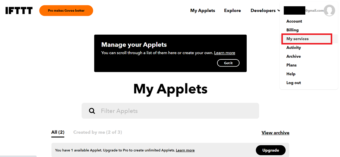


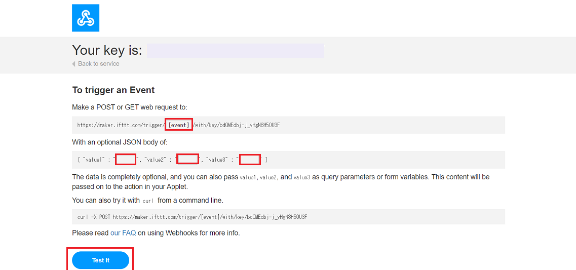


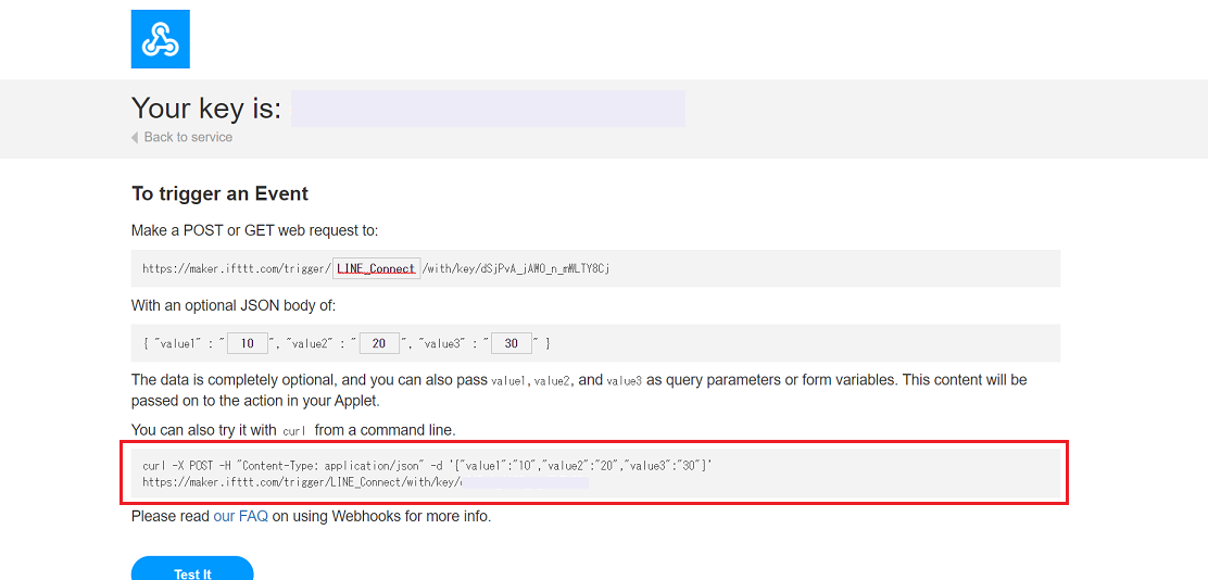

- 投稿日:2021-03-01T15:46:05+09:00
Twitterで人工地震と検索してマルコフ連鎖でランダムな文章を生成してTweetする
こんなbotが出来た
- 人工地震で検索して、マルコフ連鎖で文章生成して、30分に1回ツイートする。
なんで作った
- 地震が起きるたびに人工地震がトレンドに上がるのをきっかけに、癒しを求めて人工地震、ディープステート、ケムトレイルなどで検索して楽しんでいたのだが、大体のコレ系は文体が似通っていることが多く、しゅうまいくんのようなマルコフ連鎖で似たような文章を無限に作れるのでは?と思ったのがきっかけである。
コード
生成する文章の元をツイートを検索して収集
- 文章生成の元となるツイートを検索する
- URLはマルコフ連鎖の関数に入れたときに良く分からないKeyErrorになることが多いので除去している。RTを除くのは同一内容を除くため、リプライを除くのは事故を防ぐためである。
- ツイートのURLがツイートに含まれると引用RTになってしまう。 引用RTはある意味ソレ系ツイートっぽいので気分でONOFFを切り替えている。
- なんとなく100回にしている。
def tweet_search(search_words):
    auth = tweepy.OAuthHandler(consumer_key, consumer_secret)
    auth.set_access_token(access_key, access_secret)
    api = tweepy.API(auth)
    set_count = 100
    word = search_words
    results = api.search(q=word, count=set_count)
    strResult = ""
    for result in results:
        # if "RT" not in result.text and "@" not in result.text:
        if "RT" not in result.text and "@" not in result.text and "https://t.co/" not in result.text:
            strResult += result.text
    print("-----Generate text based on this text-----")
    print(strResult)
    return strResult
janomeを利用して取得したツイートを単語単位に分割する
def wakati(text):
   text = text.replace('\n','')
   text = text.replace('\r','')
   t = Tokenizer()
   result =t.tokenize(text, wakati=True)
   print("-----Generate words list-----")
   print(result)
   return result
分割した単語から文章を自動作成する
- ここのコードを丸パクリしていていたが、KeyErrorの無限ループにハマったので、breakで抜けるようにした。
- 正直、何で動くのか、何となくでしか理解していない。
def generate_text(words_list):
   num_sentence = 5 # ここを変更すると何度も文章を作成する
   words_list = words_list

   markov = {}
   w1 = ""
   w2 = ""
   for word in words_list:
       if w1 and w2:
           if (w1, w2) not in markov:
               markov[(w1, w2)] = []
           markov[(w1, w2)].append(word)
       w1, w2 = w2, word

   count_kuten = 0 #  "。"
   num_sentence = num_sentence
   sentence = ""
   w1, w2  = random.choice(list(markov.keys()))
   while count_kuten < num_sentence:
       try:
           tmp = random.choice(markov[(w1, w2)])
           sentence += tmp
       except KeyError: # 問題個所
           break
       except Exception as e:
           print(e)
           print(type(e))
       if(tmp=='。'):
           count_kuten += 1
           sentence += '\n'
       w1, w2 = w2, tmp

   print("-----Generated Text-----")
   print(sentence)

   return sentence
実行部分
- 汎用性を高めるために引数で検索語句を受け付けて、上記の関数に渡しているだけである。crontabに
-w "人工地震"と記述する。if __name__ == "__main__": search_words = [] parser = argparse.ArgumentParser(description='search words(space separated)') parser.add_argument('-w','--words',metavar='words',type=str,help='search words(space separated)',default="") args = parser.parse_args() print(args) if args.words == "": print("No Argument") sys.exit() s = args.words search_words = s.split() print(search_words) # Search for tweets data and generate text tweet_text = generate_text(wakati(tweet_search(search_words))) # trim tweet_text_140 = tweet_text[1:140] print("-----Text trimmed to 140 characters-----") print(tweet_text_140) auth = tweepy.OAuthHandler(consumer_key, consumer_secret) auth.set_access_token(access_key, access_secret) api = tweepy.API(auth) # tweet try: api.update_status(tweet_text_140) except Exception as e: print(e) print(type(e))全部入りのコード
- Githubにあげてある
- TwitterのAPIKeyをpublicな場所にアップロードすると、冷や汗だらだらになるので気をつけましょう
参考にした記事
- Tweepy で Twitter の単語を検索する
- Pythonでマルコフ連鎖で文章生成してみる
- ほぼほぼここのコードの改良版なので足を向けて寝られない
- APIキーなどの環境変数を管理
- ベタ書きは推奨されていないらしく
- SWAP領域の確認と作成
- GCPの無料枠で動かしているのでメモリが一瞬で枯渇しました
感想
- マルコフ連鎖はしゅうまいくんみたいなものという認識しかなかったのに、コードを拾ってくる検索スキルだけで似たようなものが作れるというのに感動した。コードを読めるようにしないといけないのは重々わかるのだが、動いてしまったのだから仕方ない。
- 今後やりたいこと
- cronで動かしてるだけで、全くログを取っていないので、ログを取る。
- 母数を貯めていって学習している風にする。
- 投稿日:2021-03-01T15:46:05+09:00
Twitterで任意の言葉を検索してマルコフ連鎖でランダムな文章を生成してTweetする
こんなbotが出来た
- 人工地震で検索して、マルコフ連鎖で文章生成して、30分に1回ツイートする。
なんで作った
- 地震が起きるたびに人工地震がトレンドに上がるのをきっかけに、癒しを求めて人工地震、ディープステート、ケムトレイルなどで検索して楽しんでいたのだが、大体のコレ系は文体が似通っていることが多く、しゅうまいくんのようなマルコフ連鎖で似たような文章を無限に作れるのでは?と思ったのがきっかけである。
コード
生成する文章の元をツイートを検索して収集
- 文章生成の元となるツイートを検索する
- URLはマルコフ連鎖の関数に入れたときに良く分からないKeyErrorになることが多いので除去している。RTを除くのは同一内容を除くため、リプライを除くのは事故を防ぐためである。
- ツイートのURLがツイートに含まれると引用RTになってしまう。 引用RTはある意味ソレ系ツイートっぽいので気分でONOFFを切り替えている。
- なんとなく100回にしている。
def tweet_search(search_words): auth = tweepy.OAuthHandler(consumer_key, consumer_secret) auth.set_access_token(access_key, access_secret) api = tweepy.API(auth) set_count = 100 word = search_words results = api.search(q=word, count=set_count) strResult = "" for result in results: # if "RT" not in result.text and "@" not in result.text: if "RT" not in result.text and "@" not in result.text and "https://t.co/" not in result.text: strResult += result.text print("-----Generate text based on this text-----") print(strResult) return strResultjanomeを利用して取得したツイートを単語単位に分割する
def wakati(text): text = text.replace('\n','') text = text.replace('\r','') t = Tokenizer() result =t.tokenize(text, wakati=True) print("-----Generate words list-----") print(result) return result分割した単語から文章を自動作成する
- ここのコードを丸パクリしていていたが、KeyErrorの無限ループにハマったので、breakで抜けるようにした。
- 正直、何で動くのか、何となくでしか理解していない。
def generate_text(words_list): num_sentence = 5 # ここを変更すると何度も文章を作成する words_list = words_list markov = {} w1 = "" w2 = "" for word in words_list: if w1 and w2: if (w1, w2) not in markov: markov[(w1, w2)] = [] markov[(w1, w2)].append(word) w1, w2 = w2, word count_kuten = 0 # "。" num_sentence = num_sentence sentence = "" w1, w2 = random.choice(list(markov.keys())) while count_kuten < num_sentence: try: tmp = random.choice(markov[(w1, w2)]) sentence += tmp except KeyError: # 問題個所 break except Exception as e: print(e) print(type(e)) if(tmp=='。'): count_kuten += 1 sentence += '\n' w1, w2 = w2, tmp print("-----Generated Text-----") print(sentence) return sentence実行部分
- 引数で検索語句を受け付けて、上記の関数に渡しているだけである。
if __name__ == "__main__":
    search_words = []
    parser = argparse.ArgumentParser(description='search words(space separated)')
    parser.add_argument('-w','--words',metavar='words',type=str,help='search words(space separated)',default="")
    args = parser.parse_args()
    print(args)
    if args.words == "":
        print("No Argument")
        sys.exit()
    s = args.words
    search_words = s.split()
    print(search_words)
    # Search for tweets data and generate text
    tweet_text = generate_text(wakati(tweet_search(search_words)))
    # trim
    tweet_text_140 = tweet_text[1:140]
    print("-----Text trimmed to 140 characters-----")
    print(tweet_text_140)
    auth = tweepy.OAuthHandler(consumer_key, consumer_secret)
    auth.set_access_token(access_key, access_secret)
    api = tweepy.API(auth)
    # tweet
    try:
        api.update_status(tweet_text_140)
    except Exception as e:
        print(e)
        print(type(e))
全部入りのコード
- Githubにあげてある
- TwitterのAPIKeyをpublicな場所にアップロードすると、冷や汗だらだらになるので気をつけましょう
参考にした記事
- Tweepy で Twitter の単語を検索する
- Pythonでマルコフ連鎖で文章生成してみる
- ほぼほぼここのコードの改良版なので足を向けて寝られない
- APIキーなどの環境変数を管理
- ベタ書きは推奨されていないらしく
- SWAP領域の確認と作成
- GCPの無料枠で動かしているのでメモリが一瞬で枯渇しました
感想
- マルコフ連鎖はしゅうまいくんみたいなものという認識しかなかったのに、コードを拾ってくる検索スキルだけで似たようなものが作れるというのに感動した。コードを読めるようにしないといけないのは重々わかるのだが、動いてしまったのだから仕方ない。
- 今後やりたいこと
- cronで動かしてるだけで、全くログを取っていないので、ログを取る。
- 母数を貯めていって学習している風にする。
- 投稿日:2021-03-01T15:12:22+09:00
Dashでウェブアプリ作成①
はじめに
データの基礎分析や分類モデルなどを作成したものをアプリ上で見せたり触ったりできると嬉しいと思い、lotlyが提供している可視化フレームワークであるDashを扱ってみる。Dash Documentation & User Guide | Plotlyのチュートリアルを参考に進める。
実行環境
以下環境で実行した。
- Windows10 Pro
- Anaconda 4.9.2
- Python 3.7.6
- dash 1.19.0
- dash-core-components 1.15.0
- dash-html-components 1.1.2Dashは以下コマンドでインストールした。
install.pyconda install -c conda-forge dashデータテーブルの可視化
チュートリアルDash Layoutに従って、以下コードを実行する。
table.py# Run this app with `python app.py` and # visit http://127.0.0.1:8050/ in your web browser. import dash import dash_html_components as html import pandas as pd df = pd.read_csv('https://gist.githubusercontent.com/chriddyp/c78bf172206ce24f77d6363a2d754b59/raw/c353e8ef842413cae56ae3920b8fd78468aa4cb2/usa-agricultural-exports-2011.csv') def generate_table(dataframe, max_rows=10): return html.Table([ html.Thead( html.Tr([html.Th(col) for col in dataframe.columns]) ), html.Tbody([ html.Tr([ html.Td(dataframe.iloc[i][col]) for col in dataframe.columns ]) for i in range(min(len(dataframe), max_rows)) ]) ]) external_stylesheets = ['https://codepen.io/chriddyp/pen/bWLwgP.css'] app = dash.Dash(__name__, external_stylesheets=external_stylesheets) app.layout = html.Div(children=[ html.H4(children='US Agriculture Exports (2011)'), generate_table(df) ]) if __name__ == '__main__': app.run_server(debug=True)http://127.0.0.1:8050/に接続すると、以下のようなテーブルが可視化される。
上記をベースに、統計量の表示などが別タブで見られるように調査しながらカスタマイズしていく。データはdefault of credit card clients Data Setを使用する。
タブの追加
上記のような生データ自体を見るページとは別に基礎統計量などを見られるようにしたいと考えたため、別タブの追加を検討する。別タブの追加には、dash-core-components(以下dcc)にてdcc.Tabまたはdcc.Tabsが使用できる。dcc.Tabは個々のタブのスタイルと値を扱い、dcc.Tabsはdcc.Tabコンポーネントの集合を扱うとのこと。dcc.Tab Reference、Tabs Examples and Referenceを参考に単純にタブを追加してみる。以下に修正したコードを示す。使用しているデータには、Rで基礎分析結果をCSV出力①全体編, Rで基礎分析結果をCSV出力②量的変数編で作成したCSVファイルを用いている。
addTab.py# Run this app with `python app.py` and # visit http://127.0.0.1:8050/ in your web browser. import dash import dash_html_components as html import dash_core_components as dcc import pandas as pd from dash.dependencies import Input, Output df1 = pd.read_csv( "c:/***/default_of_credit_card_clients.csv", header=1) df1.columns.values[0] = '' df2 = pd.read_csv( "c:/***/summary.csv", header=0) df2.columns.values[0] = '' df3 = pd.read_csv( "c:/***/stats.csv", header=0) df3.columns.values[0] = '' def generate_table(dataframe, max_rows=10): return html.Table([ html.Thead( html.Tr([html.Th(col) for col in dataframe.columns]) ), html.Tbody([ html.Tr([ html.Td(dataframe.iloc[i][col]) for col in dataframe.columns ]) for i in range(min(len(dataframe), max_rows)) ]) ]) external_stylesheets = ['https://codepen.io/chriddyp/pen/bWLwgP.css'] app = dash.Dash(__name__, external_stylesheets=external_stylesheets) app.layout = html.Div([ html.H4(children='default of credit card clients Data Set'), dcc.Tabs(id='tabs-example', value='tab-1', children=[ dcc.Tab(label='raw data', value='tab-1'), dcc.Tab(label='number of missing values', value='tab-2'), dcc.Tab(label='stats', value='tab-3') ]), html.Div(id='tabs-example-content'), ]) @app.callback(Output('tabs-example-content', 'children'), Input('tabs-example', 'value')) def render_content(tab): if tab == 'tab-1': return html.Div([ generate_table(df1) ]) elif tab == 'tab-2': return html.Div([ generate_table(df2, max_rows=30) ]) elif tab == 'tab-3': return html.Div([ generate_table(df3, max_rows=20) ]) if __name__ == '__main__': app.run_server(debug=True)結果は以下のようになる。
おわりに
チュートリアルを参考に、別タブを追加してそれぞれのタブでデータを表示できた。次の記事では、図を作成し表示させてみる。
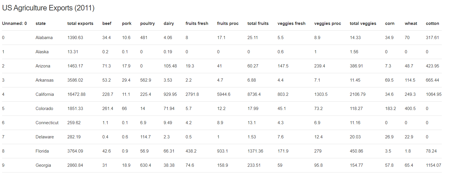
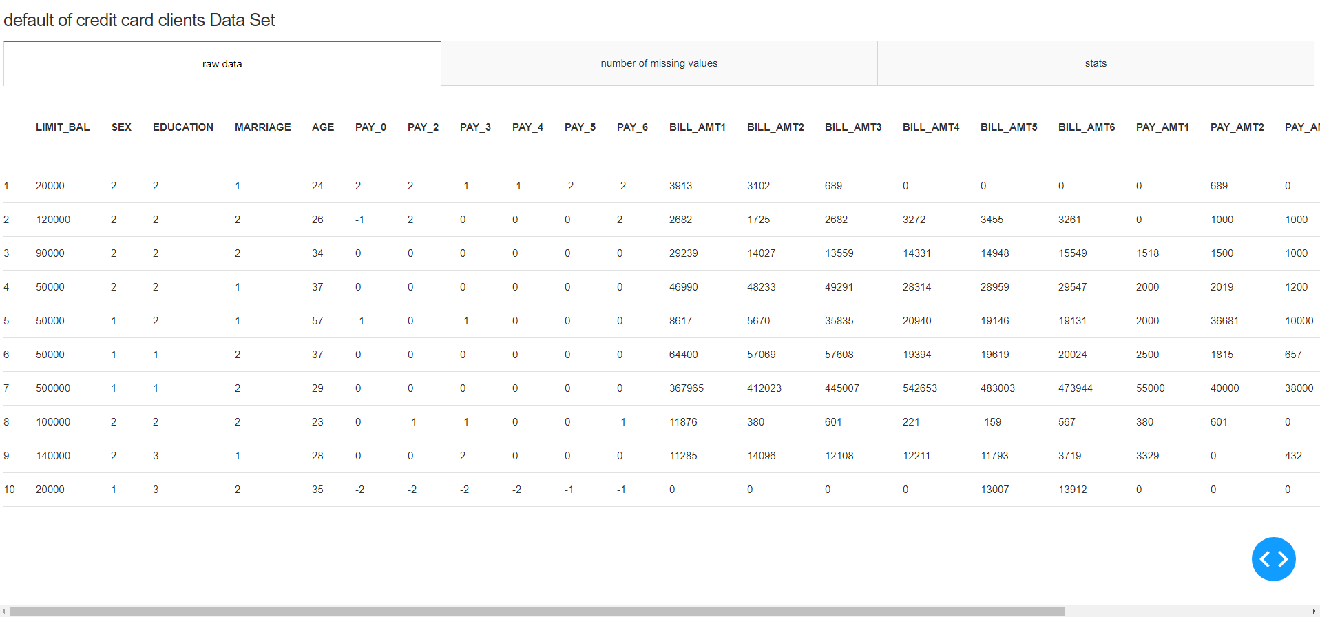
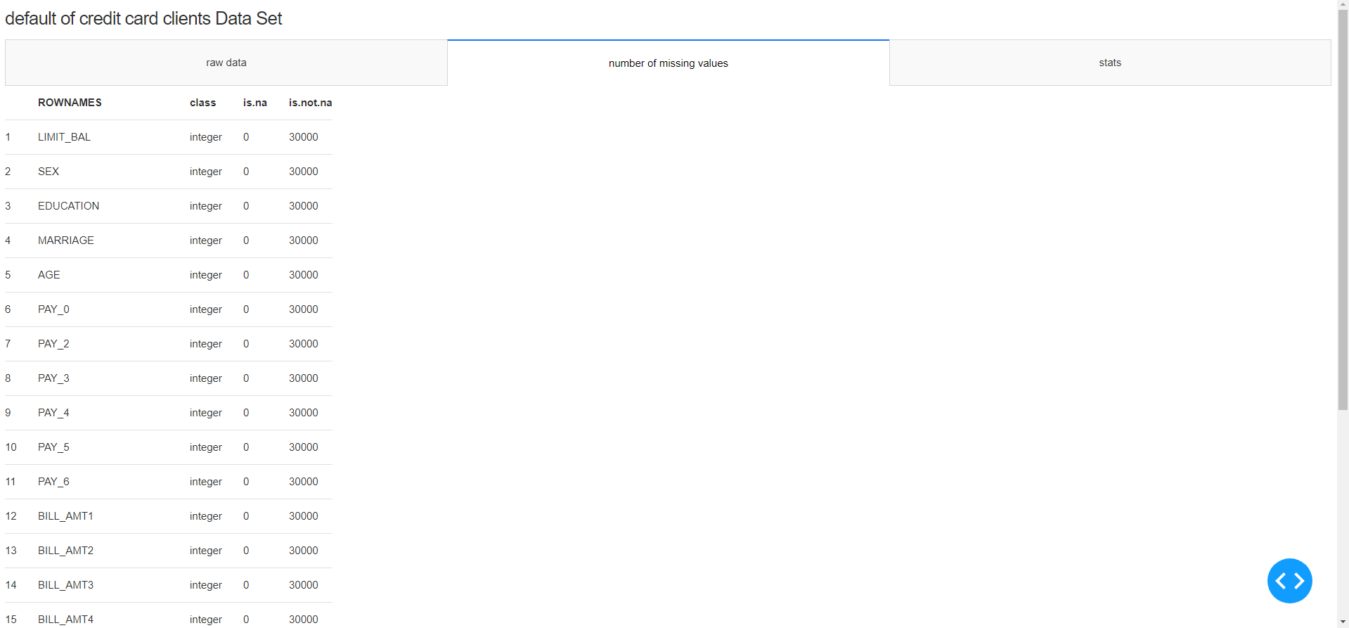
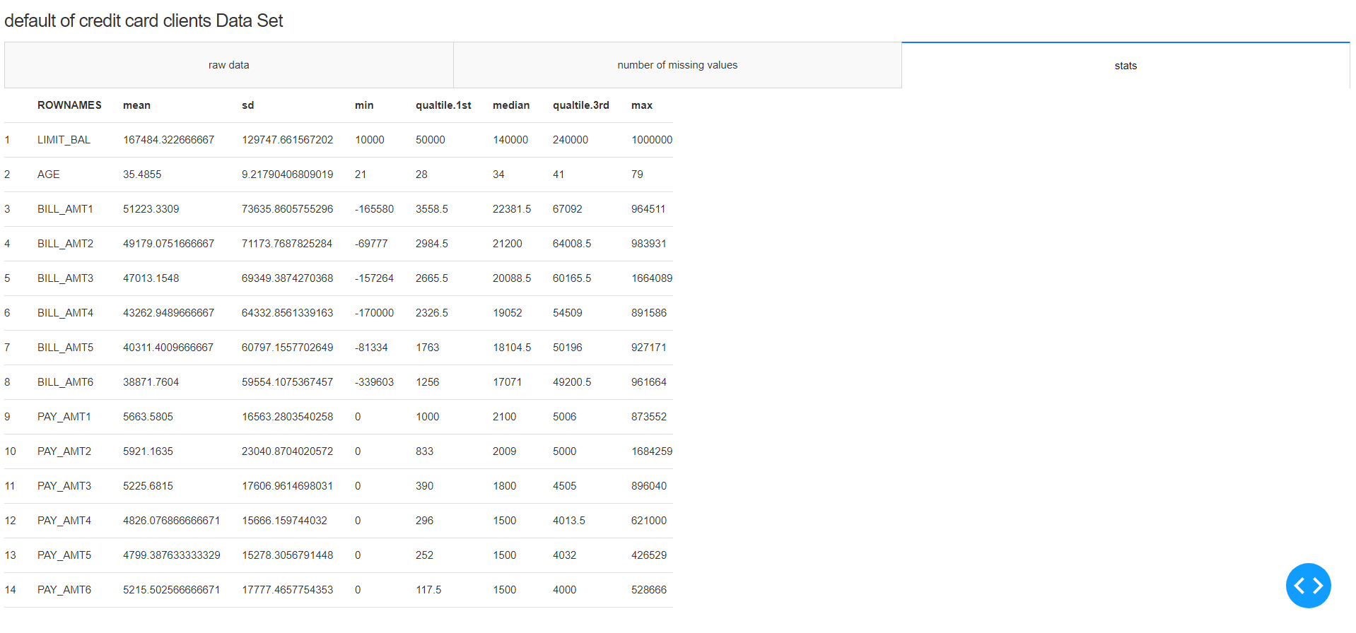
- 投稿日:2021-03-01T15:01:45+09:00
ffmpegでスライドショーをやろうとして嵌まった
ffmpegでスライドショーをやろうとして嵌まった
覚書メモです
予め画像は解像度を合わせておく
tarなりでバックアップを取った後、magickを使って変換する
find ./*.jpg -exec magick convert {} -resize 1920x1080 -background black -gravity center -extent 1920x1080 {} \;ffmpegのコマンドラインが地獄
from glob import glob
from subprocess import run

clips = glob("./*.jpg") # 画像リスト
clips.sort()

output = "video.mp4" # 出力ファイル名
cliptime = 16 # 画像クリップの表示時間
duration = 2  # クロスフェード時間

# クロスフェードで重なる分、次のクリップの再生が早まる
# step * len(clips) + duration が最終的な尺になる
step = cliptime - duration

cmd = "ffmpeg "
for clip in clips:
    # 画像クリップを表示時間分のループ素材として並べる
    cmd += "-loop 1 -t %d -i %s " % (cliptime, clip)

# クロスフェードのオプション設定、クロスフェード時間は固定なのでここで指定
xfade = "xfade=transition=fade:duration=%d" % (duration) + ":offset=%d"
cmd += "-filter_complex " # 以降フィルタ設定をしていく

pos = 0
for num in range(len(clips)-1):
    pos += step # クリップ素材のスタート位置はステップ分を累積していく
    if num == 0:
        # 一番最初は素材0と素材1を結合する
        header = "[0][1]"
    else:
        # それ以降は[v番号]の結合済み素材と次のクリップ素材を結合
        header = "[v%d][%d]" % (num, num+1)
    if num == len(clips)-2:
        # 最後の素材を結合したら[v]ラベルを付けてそれを終端にする
        footer = "[v] -map [v] -vcodec h264 -pix_fmt yuv420p %s" % (output)
    else:
        # 結合するたびに[v+後ろの素材番号]のラベルを付ける
        footer = "[v%d]\;" % (num+1)
    # コマンドラインをつなぎ合わせていく
    cmd += header + xfade % (pos) + footer

run(cmd, shell=True) # ffmpegコマンドラインの呼び出し
- 投稿日:2021-03-01T14:52:52+09:00
rpy2のインストール(Windows向け )
rpy2とはPythonからRを実行できるようにするライブラリーです。
Windowsでのrpy2のインストール方法が説明されているサイトが無かったので作成しました。
pipで簡単にできましたが、逆に出来ないとか苦労したとかいうサイトがあふれています。なぜそのような混乱が生じているのかはわかりませんが。環境
- rpy2: 3.4.2
- OS: Windows 10 May 2020 Update(バージョン2004)
- Python: 3.8.8 (Anaconda)
- R: 4.0.4
Rがないとパッケージのインストールに失敗します。また、インストール時にバージョン情報をレジストリーに登録しましたが、Rのパスは環境変数に設定していません。
pipでインストール
公式のドキュメントには「Windowsの人はDocker使ってね キラッ☆」と書かれていますが、他のパッケージと同様
pipでインストールできます。( 彡()() なんで最初にこれを試さなかったか… )PowerShell> pip install rpy2オフライン環境の場合は、
rpy2をPyPI - rpy2 download filesからダウンロードしたソース ファイル(rpy2-3.4.2.tar.gz)のパスで置き換えます。必要に応じてtzlocalも手動でインストールします。試しに以下を実行してみます。ちゃんと円周率の値が出れば成功です。
pythonimport rpy2.robjects as robjects pi = robjects.r['pi'] print(pi[0]) #3.141592653589793が出ればOKcondaでインストール
これで終わりだとつまらないので、「Anacondaなのでpipを使うのは…」と思った方のために、もう一つネタを追加します。
condaの場合は、
conda install rpy2だと失敗するため、
こちらを参考に、以下のコマンドでPyPIのソースコードからcondaパッケージを作成してインストールします:Anaconda_Poershell_Prompt> conda install -n base conda-build # ビルドに必要なパッケージのインストール > conda skeleton pypi rpy2 # スケルトン作成 > conda build rpy2 # ビルド > conda install パッケージのパスパッケージのパスは
(Anacondaインストール先)/conda-bld/win-64/rpy2-3.4.2-py38_0.tar.bz2です、たぶん。私が実行したときには、3つめのコマンドで、ビルド後のテスト中に以下のエラーが出たため、パッケージのパスが(Anacondaインストール先)/conda-bld/broken/rpy2-3.4.2-py38_0.tar.bz2になってしまいました。ipython入っているのになぜエラーが出るのか。。。(略) ModuleNotFoundError: No module named 'IPython' (%PREFIX%) %SRC_DIR%>IF 1 NEQ 0 exit /B 1 Tests failed for rpy2-3.4.2-py38_0.tar.bz2 - moving package to C:\ProgramData\Anaconda3\conda-bld\broken (略) TESTS FAILED: rpy2-3.4.2-py38_0.tar.bz2Pythonで
rpy2.robjectsのインポート時に以下のエラーが出たら、tzlocalをcondaでインストールします。ModuleNotFoundError: No module named 'tzlocal'蛇足:.whlファイル作成 & pipでインストール
この部分は蛇足です。ソースコードから.whlファイルをビルドしてインストールする方法を説明します。
- PYPI - rpy2 download Filesからソース ファイルをダウンロード
- 7-Zipなどで.tar.gzファイルを解凍
- Powershellで以下のコマンドを実行
PowerShell> cd 解凍先フォルダー # 解凍先フォルダーはsetup.pyがあるフォルダー > python setup.py bdist_wheel # パッケージ作成。`dist`フォルダーにrpy2-3.4.2-py3-non-any.whlができる。 > pip install ./dist/rpy2-3.4.2-py3-non-any.whl # インストール > pytest --pyargs 'rpy2.tests'最後のテストで以下が出てきますが、たぶん大丈夫です。
(略)
=================================================================== short test summary info ====
FAILED rinterface/test_vector_str.py::test_non_asciil - UnicodeDecodeError: 'utf-8' codec can't
======================================== 1 failed, 696 passed, 64 skipped, 4 xfailed, 1 xpassed,
(略)
試してみて失敗したこと
非公式バイナリーからのインストール
非公式バイナリーはrpy2 2.9.5, Python 3.7で更新が止まっているため、Python 3.8には使えませんでした。公式のドキュメントにも以前は非公式バイナリーの紹介がありましたが、現在(3.4.x)はなくなっています。
conda-forgeからインストール
condaのチャネルにconda-forgeを追加して、
codnda install rpy2を実行してみましたが、Python 3.8以上だとダメでした。ソースコードのC言語部分だけをビルド
リンクエラーが出まくりました。そもそもCのビルドは必要ありませんでした(.whlファイルにそれっぽいものが含まれていない)。
参考
- 公式ドキュメント v3.4.x Installation
- Condaパッケージの作成方法
- rpy2導入時に発生した問題点
- Compile `rpy2` (API mode) on Windows #624
- Rpy2の使い方の備忘録
全く気乗りしないけどRの勉強を始めるか
('A`)...
- 投稿日:2021-03-01T14:42:34+09:00
『PythonとJavaScriptではじめるデータビジュアライゼーション』がとても良い本なので
この記事は?
題名に書いたオライリー・ジャパンから出ている本、とてもいいのですがいかんせん古い。
そのため、書籍通りにコーディングしても100%うまくいきません。なので2021年2月時点でこう書けばうまく動く、というのを備忘録的に残しておきます。
PythonとJavaScriptではじめるデータビジュアライゼーション
対象の箇所
6章「Scrapyを使った重量スクレイピング」の
nwinners_list_spider.py
です。wikipediaの構造が変わっているのでxpathが書籍の執筆時点と異なります。
それを考慮して、次のようにコーディングするとうまく動きました。(ノーベル賞受賞者のリストが取れた!)import scrapy import re BASE_URL = 'https://en.wikipedia.org' class NWinnerItem(scrapy.Item): name = scrapy.Field() link = scrapy.Field() year = scrapy.Field() category = scrapy.Field() country = scrapy.Field() gender = scrapy.Field() born_in = scrapy.Field() date_of_birth = scrapy.Field() date_of_death = scrapy.Field() place_of_birth = scrapy.Field() place_of_death = scrapy.Field() text = scrapy.Field() class NWinnerSpider(scrapy.Spider): name = 'nwinners_full' allowd_domains = ['en.wikipedia.org'] start_urls = [ 'https://en.wikipedia.org/wiki/List_of_Nobel_laureates_by_country' ] def parse(self, response): filename = response.url.split('/')[-1] h3s = response.xpath('//h3') for h3 in h3s: country = h3.xpath('span[@class="mw-headline"]/text()').extract() if country: winners = h3.xpath('following-sibling::ol[1]') for w in winners.xpath('li'): wdata = process_winner_li(w, country[0]) request = scrapy.Request( wdata['link'], callback=self.parse_bio, dont_filter=True ) request.meta['item'] = NWinnerItem(**wdata) yield request def parse_bio(self, response): item = response.meta['item'] href = response.xpath("//li[@id='t-wikibase']/a/@href").extract() if href: url = href[0] request = scrapy.Request(href[0],callback=self.parse_wikidata,dont_filter=True) request.meta['item'] = item yield request def parse_wikidata(self, response): item = response.meta['item'] property_codes = [ {'name': 'date_of_birth', 'code':'P569'}, {'name': 'date_of_death', 'code':'P570'}, {'name': 'place_of_birth', 'code': 'P19', 'link':True}, {'name': 'place_of_death', 'code': 'P20', 'link':True}, {'name': 'gender', 'code':'P21', 'link': True} ] p_template = '//*[@id="{code}"]/div[2]/div/div[1]/div[2]/div[1]/div/div[2]/div[2]/div[1]/{link_html}/text()' for prop in property_codes: link_html = '' if prop.get('link'): link_html = '/a' sel = response.xpath(p_template.format(code=prop['code'], link_html=link_html)) if sel: item[prop['name']] = sel[0].extract() yield item def process_winner_li(w, country=None): wdata = {} wdata['link'] = BASE_URL + w.xpath('a/@href').extract()[0] text = ' '.join(w.xpath('descendant-or-self::text()').extract()) wdata['name'] = text.split(',')[0].strip() year = re.findall('\d{4}', text) if year: wdata['year'] = int(year[0]) else: wdata['year'] = 0 print('Oops, NO YEAR in ', text) category = re.findall('Physics|Chemistry|Physiology or Medicine|Literature|Peace|Economics', text) if category: wdata['category'] = category[0] else: wdata['category'] = '' print('NO CATEGORY in ', text) if country: if text.find('*') != -1: wdata['country'] = '' wdata['born_in'] = country else: wdata['country'] = country wdata['born_in'] = '' wdata['text'] = text return wdata以上です。
個人的な備忘録ですので、ご利用の際はご注意ください。
- 投稿日:2021-03-01T14:29:08+09:00
Pandas入門
You can find the English version of this article here ⇒ Pandas Fundamentals
はじめに
今回の投稿の目的は、PythonライブラリであるPandasの基本的な機能と使い方を説明することです。
概要
Pandasは表形式のデータ(例:表計算やデータベースのデータ)を処理するためのPythonライブラリです。
データ分析や、機械学習の分野でよく使われます。
インストール
最新版は
pipを用いてインストールすることができます。pip install pandas概念
まずは、ライブラリで使われている概念や用語を説明しておきましょう。
Series(シリーズ)
Seriesはリストのような一次元のデータ構造であり、色々なデータ型が格納できます(
int,float,dict等)
DataFrame(データフレーム)
- テーブルのように複数行と列をもつ2次元のデータ構造である
- 各カラムをSeriesと考えることができる
- 概念的にスプレッドシートまたデータベーステーブルに類似している
今回の投稿では、DataFrameの使い方に最も注目していきます。
DataFrame作成
多くの場合、ファイルやデータベースから既存のデータを読み込むことでDataFrameを作成します。
たとえば、CSV(カンマ区切り形式)ファイルを読み込むには、次のようにします。
import pandas as pd
df = pd.read_csv('example.csv')
df
また、Pythonの
dictオブジェクトからDataFramesを作成することもできます。import pandas as pd data = {'A': [1, 2, 3], 'B': ['X', 'Y', 'Z'], 'C': [0.1, 0.2, 0.3]} df = pd.DataFrame(data) >>> df A B C 0 1 X 0.1 1 2 Y 0.2 2 3 Z 0.3カラムのデータをアクセスする
DataFrame内のデータにアクセスする方法を見てみましょう。
以下のDataFrameを例として使います。
1つのカラムのデータにアクセスするには、主に2つの方法があります。
複数のカラムのデータにアクセスするにはカラム名のリストを入れます。
インデックス
次に、「インデックス」とは何か、どのように使えるのかを説明します。
DataFrameまたはSeriesの行と列を選択するために使用します。
インデックスにアクセスするには、主に3つの方法があります。
locは特定のラベルを持つ列または行を取得するilocは特定の位置で行または列を取得するixは通常、locのように動作しようとしますが、ラベルがインデックスに存在しない場合、ilocのように動作します。 (非推奨なのでlocまたはilocを使用してください)注:インデックスで数値ラベルがよく使用されるため、行を選択したときに
ilocとlocが同じ結果を返す可能性がある。 ただし、インデックスの順序が変更された場合(データがソートされた場合など)、結果は同じにならない可能性もあるそれでは、
locが使われている使用事例を見てみましょう。
それでは、
ilocを使って同じデータを選択してみましょう。
多くの場合、インデックスには数値ラベルが使用されるので、行を選択する際に
ilocとlocが同じ結果を返すことがあります。しかし、以下の例のようにインデックスの順序が変更されている場合、結果は同じではないかもしれません。
data = {'Col1': ['A', 'B', 'C', 'D'], 'Col2': [1, 2, 3, 4]} df = pd.DataFrame(data) >>> df Col1 Col2 0 A 1 1 B 2 2 C 3 3 D 4DataFrameを
Col2で並べ替えると、データの位置が変わるので、locとilocの結果が異なります。df.sort_values('Col2', ascending=False) Col1 Col2 3 D 4 2 C 3 1 B 2 0 A 1条件付きステートメント
条件付きステートメントを適用することにより、DataFrameの一部を選択できます。 これには2つの方法があります。
複数の条件を使用している場合は、それぞれの条件を括弧で囲む必要があることに注意してください。
例えば、これの代わりに
df[df.Col1 == 'A' | df.Col2 == 2] >>> TypeError: cannot compare a dtyped [int64] array with a scalar of type [bool]次のようにします。
>>> df[(df.Col1 == 'A') | (df.Col2 == 2)] Col1 Col2 0 A 1 1 B 2算術演算
代入を実行することで、DataFrame の内容を変更することができます。
また、以下の例にあるように、DataFrameに対して算術演算を行うこともできます。
算術演算は変更したDataFrameのコピーを返す
例として、Data Frame,
dfを変更しましょうdata = {'Col1': ['A', 'B', 'C', 'D'], 'Col2': [1, 2, 3, 4], 'Col3': [1, 2, 3, 4]} df = pd.DataFrame(data) >>> df Col1 Col2 Col3 0 A 1 1 1 B 2 2 2 C 3 3 3 D 4 4まずは1つのセルの値を掛け合わせてみましょう。
>>> df.loc[0, 'Col2'] * 2 2次に、
Col3のすべての値から1を引いてみましょう。df['Col3'] - 1 0 0 1 1 2 2 3 3 Name: Col3, dtype: int64次に、
Col3のすべての値に1を足して、その結果を元のDataFrameに代入してみましょう。df['Col3'] += 1 >>> df Col1 Col2 Col3 0 A 1 2 1 B 2 3 2 C 3 4 3 D 4 5最後に、
Col3の値が3より大きい場合にCol2に0の値を代入する条件を用いてみましょう。df.loc[df.Col3 > 3, 'Col2'] = 0 >>> df Col1 Col2 Col3 0 A 1 2 1 B 2 3 2 C 0 4 3 D 0 5よく使う関数
Pandasは算術演算に加えて、DataFrameの処理を簡単にするための多くの関数を提供されています。
いくつかよく使う関数を紹介します。
関数名 目的 使用事例 df.dropna() 空値「NaN」のもつ行を外す df = df.dropna() df.fillna() 指定された値で空値のもつ列をデフォルトする df = df.fillna(1) df.rename() 列の名前を変更する df.rename(columns={‘old’: ‘new’}) df.sort_values() 列でデータをソートする df.sort_values(by=[’col1’]) df.describe() 列の統計情報を表示する (平均値, 最大値, 最小値, 等) df.col1.describe() 参考資料
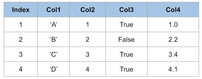
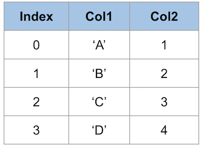

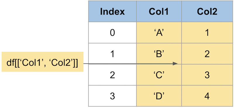


- 投稿日:2021-03-01T14:28:20+09:00
Pandas Fundamentals
この記事の日本語版はこちら ⇒ Pandas入門
Introduction
The purpose of the this post is to explain the fundamentals of using the Pandas library for Python.
Overview
Pandas is a Python library that is used to manipulate tabular data (similar to the data in a spreadsheet or database).
It is often used for data analysis and for reading and manipulating datasets used by Machine Learning libraries.
Installation
The latest version can be installed using
pip:pip install pandasConcepts
To begin with, let's understand the concepts and terminology used by the library.
Series
A Series is a single-dimensioned labeled array that is able to hold any type of data.
DataFrame
A DataFrame is a two-dimensional table-like data structure with multiple rows and columns.
- You can consider it as a collection of Series.
- Similar in concept to a spreadsheet or database table.

In this post, we will focus most of our attention on how to use DataFrames.
Creating a DataFrame
Often, you will create a DataFrame by loading existing data from a file, or database. For example, to load a CSV (comma-separated values) file:
import pandas as pd df = pd.read_csv('example.csv') >>> dfYou can also create DataFrames from Python dictionary objects, where each key in the dictionary corresponds to a column name.
import pandas as pd data = {'A': [1, 2, 3], 'B': ['X', 'Y', 'Z'], 'C': [0.1, 0.2, 0.3]} df = pd.DataFrame(data) >>> df A B C 0 1 X 0.1 1 2 Y 0.2 2 3 Z 0.3Accessing Columns
Now, let's look at how we access data within a DataFrame.
Given the following DataFrame,
df:
There are two main ways to access all data in a single column:
You can also select data in multiple columns:
Index
Next, let's understand what the 'index' is and how we can use it.
The index is used to select rows or columns in a DataFrame or Series.
There are three main ways to access the index:
locgets rows (or columns) with particular labels from the index.ilocgets rows (or columns) at particular positions in the index (so it only takes integers).ixusually tries to behave like loc but falls back to behaving likeilocif a label is not present in the index. (Deprecated, use loc or iloc instead)Lets have a look at some examples, starting with
loc:
Now let's select the same data using
iloc:
Often numeric labels are used in the index so it’s possible that
ilocandlocreturn the same results when selecting rows.However, if the order of the index has changed, as seen in the example below, the results may not be the same.
Given the following Data Frame,
df:data = {'Col1': ['A', 'B', 'C', 'D'], 'Col2': [1, 2, 3, 4]} df = pd.DataFrame(data) >>> df Col1 Col2 0 A 1 1 B 2 2 C 3 3 D 4After sorting the DataFrame
df, byCol2in descending order the position of the data will change:df.sort_values('Col2', ascending=False) Col1 Col2 3 D 4 2 C 3 1 B 2 0 A 1Conditions
You can apply one or more conditions to select a subset of the DataFrame. As you can see below there are a few ways of doing this:
Note that if you are using multiple conditions then you will need to enclose each condition with brackets.
For example do this:
df[(df.Col1 == 'A') | (df.Col2 == 2)]
  Col1  Col2
0    A     1
1    B     2
Instead of this:
df[df.Col1 == 'A' | df.Col2 == 2]

TypeError: cannot compare a dtyped [int64] array with a scalar of type [bool]
Arithmetic Operations and Assignment
You can modify the contents of a DataFrame by performing assignment.
You can also perform arithmetic operations on the DataFrame, as we can see in the examples below.
Note that the operations return a modified copy of the DataFrame.
Given the following Data Frame,
df:data = {'Col1': ['A', 'B', 'C', 'D'], 'Col2': [1, 2, 3, 4], 'Col3': [1, 2, 3, 4]} df = pd.DataFrame(data) >>> df Col1 Col2 Col3 0 A 1 1 1 B 2 2 2 C 3 3 3 D 4 4Let's first try and multiply the value of a single cell.
df.loc[0, 'Col2'] * 2
2
Next let's subtract
1from all values inCol3.df['Col3'] - 1 0 0 1 1 2 2 3 3 Name: Col3, dtype: int64Next let's add
1to all values inCol3and assign the result to the original DataFrame.df['Col3'] += 1 >>> df Col1 Col2 Col3 0 A 1 2 1 B 2 3 2 C 3 4 3 D 4 5Finally let's use a condition to assign a value of
0toCol2if the value inCol3is greater than3.df.loc[df.Col3 > 3, 'Col2'] = 0 >>> df Col1 Col2 Col3 0 A 1 2 1 B 2 3 2 C 0 4 3 D 0 5Common Functions
In addition to arithmetic operations Pandas also provides a large number of functions to simplify your DataFrame processing.
Here are some of the most common operations.
Operation Purpose Example df.dropna() Removes rows with NaN values df = df.dropna() df.fillna() Fills NaN values with the specified value. df = df.fillna(1) df.rename() Renames one or more columns df.rename(columns={‘old’: ‘new’}) df.sort_values() Sorts the data by one or more columns df.sort_values(by=[’col1’]) df.describe() Provides a summary of the data in the column (mean, max, min, etc) df.col1.describe() Further Reading


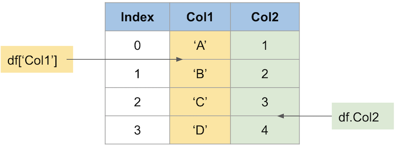

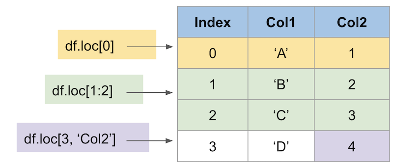
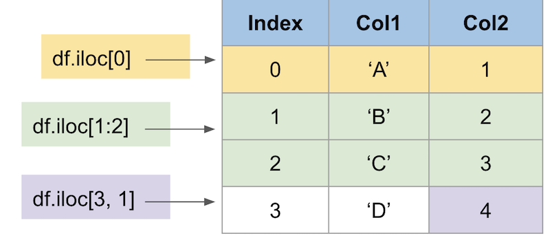
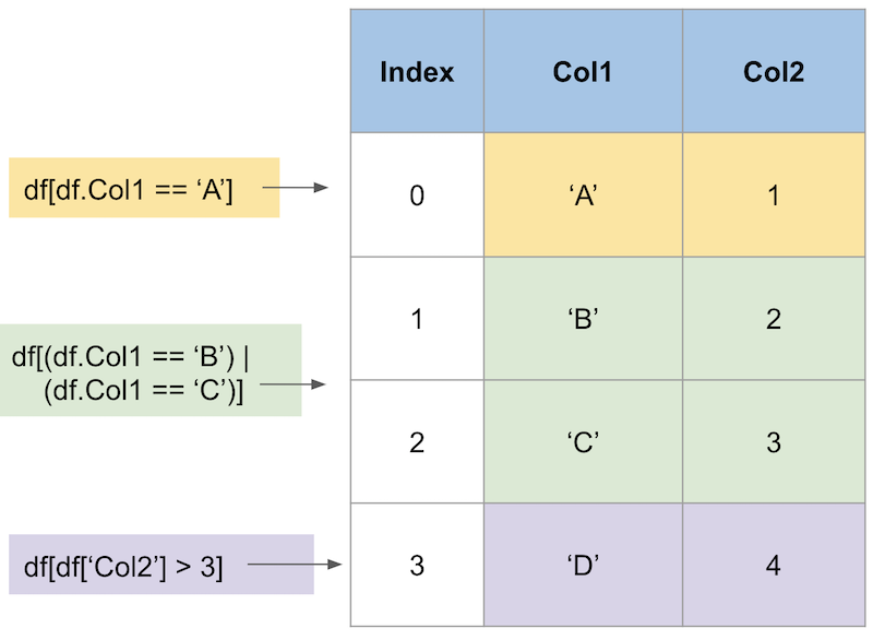
- 投稿日:2021-03-01T14:24:42+09:00
matplotlib.animationでグラフをアニメーションさせる
matplotlib.animationとは
値やデザインを変えたグラフを連続して描画することでアニメーションさせるmatplotlibの機能です。gif画像や動画ファイルで書き出したりhtml + JavaScriptで書き出すことも出来るので二次利用もやりやすいと思います。
1. インストール
matplotlibをインストールするだけです
terminalpip install matplotlib2. 2つのクラス
2つのクラスから選べます
matplotlib.animation.ArtistAnimation
描画情報のlistを作って描画するクラスですmatplotlib.animation.FuncAnimation
描画情報を更新する関数を渡して逐次実行で描画するクラスです
乱数を使って毎回違うグラフを描画するような使い方が出来ます3. 使い方
3-1. terminal実行で使う
こちらのコードをお借りしてやってみます
https://qiita.com/yubais/items/c95ba9ff1b23dd33fde21. ArtistAnimationの場合
plt.plot()などで作った描画分のオブジェクトをlistにしてArtistAnimationに放り込んでやるとアニメーション描画をやってくれます。ArtistAnimationでは先に描画情報を作っておいてから放り込むので繰り返しパターンは同じになります。
artist_animation.pyimport numpy as np import matplotlib.pyplot as plt import matplotlib.animation as animation fig = plt.figure() ims = [] for i in range(10): rand = np.random.randn(100) im = plt.plot(rand) ims.append(im) ani = animation.ArtistAnimation(fig, ims, interval=100) plt.show()terminalからpython artist_animation.pyを実行するとこんな感じのが表示される筈です
2. FuncAnimationの場合
listにして放り込むのは同じですが描画する関数を
定義して渡すことで毎回違う乱数を表示出来ますfunc_animation.pyimport numpy as np import matplotlib.pyplot as plt import matplotlib.animation as animation fig = plt.figure() def plot(data): plt.cla() rand = np.random.randn(100) im = plt.plot(rand) ani = animation.FuncAnimation(fig, plot, interval=100) plt.show()terminalからpython func_animation.pyを実行するとこんな感じのが表示される筈です。下に貼っているのは後で説明するやり方で書き出したgif画像なので同じパターンの繰り返しになっていますが、pythonが表示してくれるwindowの方はちゃんと乱数を作り直して毎回違うパターンを表示してくれる筈です。
なお、上記ではplt.cla()しているので軸が毎回作り直されていますが、変わらないように書くことも出来ます。3-2. gif画像で保存する
animationオブジェクトのsaveメソッドを使えば保存できます
func_animation.pyに1行書き足すani.save('func_animation.gif', writer='pillow')writerクラスとしてはPillow、FFMpeg、ImageMagickなどが選べますが、pipで簡単にインストール出来るPillowが手軽だと思います。
3-3. jupyter notebookに表示する
上記のplt.show()で表示するやり方はjupyter notebookでは出来ないようですが、gif画像を書き出してから表示するか、Javascript htmlに変換してIPython.display.HTMLに表示してもらう事で表示できます。またh264 encoderがある環境なら動画に変換してIPython.display.HTMLで表示するやり方も使えるようです。
https://qiita.com/fhiyo/items/0ea94b0de6cd5c76d67a1. gif画像を書き出して表示する
jupyter_notebookimport numpy as np import matplotlib.pyplot as plt import matplotlib.animation as animation from IPython.display import Image fig = plt.figure() ims = [] for i in range(10): rand = np.random.randn(100) im = plt.plot(rand) ims.append(im) ani = animation.ArtistAnimation(fig, ims, interval=100) ani.save('../artist_animation.gif', writer='pillow') plt.close() Image('../artist_animation.gif')2. Javascript htmlに変換して表示する
to_jshtml()メソッドを使うとhtml + Javascriptに変換してくれます
jupyter_notebookimport numpy as np import matplotlib.pyplot as plt import matplotlib.animation as animation from IPython.display import HTML fig = plt.figure() ims = [] for i in range(10): rand = np.random.randn(100) im = plt.plot(rand) ims.append(im) ani = animation.ArtistAnimation(fig, ims, interval=100) plt.close() HTML(ani.to_jshtml())FuncAnimationで書きたい場合は以下のようにします
jupyter_notebookimport numpy as np import matplotlib.pyplot as plt import matplotlib.animation as animation from IPython.display import HTML fig = plt.figure() N = 100 rand = np.random.randn(N) im, = plt.plot(rand) def update(frame): x = np.arange(N) y = np.random.randn(N) im.set_data(x, y) ani = animation.FuncAnimation(fig, update, interval=100) plt.close() HTML(ani.to_jshtml())4. FuncAnimationとArtistAnimationの使い分け
FuncAnimationで書いても、gif画像書き出しやJavascriptでの書き出しはひと回し生成したところまでの情報での書き出しになので乱数を繰り返し生成するというのは出来ません。実行時間はFuncAnimationで書いた方が掛かりますので、jupyter notebookで使う場合はFuncAnimationで書く意味はあまりないと思います。
- 投稿日:2021-03-01T14:01:02+09:00
'Int64Index' object has no attribute 'reshape'の解決法
はじめに
オライリージャパンの「Pyhtonではじめる機械学習」のp.238にて,citibikeの時刻データをPOSIX時刻に変換するコードで以下のようなエラーが発生した.
X = citibike.index.astype("int64").reshape(-1,1) //10**9エラー内容
AttributeError: 'Int64Index' object has no attribute 'reshape'解決法
以下のように元のコードにvaluesを加えると解決できます.
X = citibike.index.astype("int64").values.reshape(-1,1) //10**9どうも自分の持っている書籍の版が古いらしく,おそらく修正前のやつであるっぽいですね...(いろいろとエラーが多いと感じる笑)
- 投稿日:2021-03-01T13:59:18+09:00
pivot_table droplevel shift groupby mergeの例 今日の成績を前日までの成績から予測するためのデータを作る。
pivot_table droplevel groupby mergeの例 として、当日の勝敗と前X日の勝敗の集計をまとめたデータを作る。
元データ
日付 銘柄 勝敗 2021-01-01 00:00:00 M100 大勝 2021-01-02 00:00:00 M100 小勝 2021-01-03 00:00:00 M100 負 2021-01-04 00:00:00 M100 取引なし 2021-01-05 00:00:00 M100 大勝 2021-01-06 00:00:00 M100 小勝 2021-01-08 00:00:00 M100 取引なし 2021-01-01 00:00:00 M200 大勝 2021-01-02 00:00:00 M200 小勝 2021-01-03 00:00:00 M200 負 2021-01-04 00:00:00 M200 取引なし 2021-01-08 00:00:00 M200 取引なし 最終的なイメージのデータ
上記元データに 前2日の勝敗の集計を追加したデータを作成する。
勝敗 前日まで_取引なし 前日まで_大勝 前日まで_小勝 前日まで_負 ('M100', Timestamp('2021-01-01 00:00:00')) 大勝 nan nan nan nan ('M100', Timestamp('2021-01-02 00:00:00')) 小勝 0 1 0 0 ('M100', Timestamp('2021-01-03 00:00:00')) 負 0 1 1 0 ('M100', Timestamp('2021-01-04 00:00:00')) 取引なし 0 0 1 1 ('M100', Timestamp('2021-01-05 00:00:00')) 大勝 1 0 0 1 ('M100', Timestamp('2021-01-06 00:00:00')) 小勝 1 1 0 0 ('M100', Timestamp('2021-01-08 00:00:00')) 取引なし 0 1 1 0 ('M200', Timestamp('2021-01-01 00:00:00')) 大勝 nan nan nan nan ('M200', Timestamp('2021-01-02 00:00:00')) 小勝 0 1 0 0 ('M200', Timestamp('2021-01-03 00:00:00')) 負 0 1 1 0 ('M200', Timestamp('2021-01-04 00:00:00')) 取引なし 0 0 1 1 ('M200', Timestamp('2021-01-08 00:00:00')) 取引なし 1 0 0 1
手順
サンプルデータ作成
import pandas as pd
# 基本となるデータ
col=["日付" , "銘柄" , "勝敗"]

dt=[
["2021/1/1" , "M100" , "大勝" ] ,
["2021/1/2" , "M100" , "小勝" ] ,
["2021/1/3" , "M100" , "負"  ] ,
["2021/1/4" , "M100" , "取引なし" ] ,
["2021/1/5" , "M100" , "大勝" ] ,
["2021/1/6" , "M100" , "小勝"  ] ,
["2021/1/8" , "M100" , "取引なし" ] ,
["2021/1/1" , "M200" , "大勝"  ] ,
["2021/1/2" , "M200" , "小勝"  ] ,
["2021/1/3" , "M200" , "負"  ] ,
["2021/1/4" , "M200" , "取引なし"  ] ,
["2021/1/8" , "M200" , "取引なし"  ] ,
]

df0=pd.DataFrame(dt,columns=col)
df0["日付"]=pd.to_datetime(df0["日付"])
df0.sort_values(["銘柄" , "日付"] ,inplace=True)
df0.set_index("日付",inplace=True)

print(df0.to_markdown())
日付 銘柄 勝敗 2021-01-01 00:00:00 M100 大勝 2021-01-02 00:00:00 M100 小勝 2021-01-03 00:00:00 M100 負 2021-01-04 00:00:00 M100 取引なし 2021-01-05 00:00:00 M100 大勝 2021-01-06 00:00:00 M100 小勝 2021-01-08 00:00:00 M100 取引なし 2021-01-01 00:00:00 M200 大勝 2021-01-02 00:00:00 M200 小勝 2021-01-03 00:00:00 M200 負 2021-01-04 00:00:00 M200 取引なし 2021-01-08 00:00:00 M200 取引なし 前日までの勝敗の集計を作る。
#日、銘柄ごとに'勝敗'を横展開する
df1=df0.copy()
df1["cnt"]=1

df1=df1.pivot_table(index=['銘柄',"日付" ], columns='勝敗' , aggfunc="count" , fill_value=0).copy()
df1=df1.droplevel(None, axis=1)
df1.reset_index( inplace=True)
df1.set_index("日付" , inplace=True)
print(df1.to_markdown())
日付 銘柄 取引なし 大勝 小勝 負 2021-01-01 00:00:00 M100 0 1 0 0 2021-01-02 00:00:00 M100 0 0 1 0 2021-01-03 00:00:00 M100 0 0 0 1 2021-01-04 00:00:00 M100 1 0 0 0 2021-01-05 00:00:00 M100 0 1 0 0 2021-01-06 00:00:00 M100 0 0 1 0 2021-01-08 00:00:00 M100 1 0 0 0 2021-01-01 00:00:00 M200 0 1 0 0 2021-01-02 00:00:00 M200 0 0 1 0 2021-01-03 00:00:00 M200 0 0 0 1 2021-01-04 00:00:00 M200 1 0 0 0 2021-01-08 00:00:00 M200 1 0 0 0 #日、銘柄ごとに2日分の集計をする df_r=df1.groupby(["銘柄"]).rolling("2d").sum().copy() print(df_r.to_markdown())
取引なし 大勝 小勝 負 ('M100', Timestamp('2021-01-01 00:00:00')) 0 1 0 0 ('M100', Timestamp('2021-01-02 00:00:00')) 0 1 1 0 ('M100', Timestamp('2021-01-03 00:00:00')) 0 0 1 1 ('M100', Timestamp('2021-01-04 00:00:00')) 1 0 0 1 ('M100', Timestamp('2021-01-05 00:00:00')) 1 1 0 0 ('M100', Timestamp('2021-01-06 00:00:00')) 0 1 1 0 ('M100', Timestamp('2021-01-08 00:00:00')) 1 0 0 0 ('M200', Timestamp('2021-01-01 00:00:00')) 0 1 0 0 ('M200', Timestamp('2021-01-02 00:00:00')) 0 1 1 0 ('M200', Timestamp('2021-01-03 00:00:00')) 0 0 1 1 ('M200', Timestamp('2021-01-04 00:00:00')) 1 0 0 1 ('M200', Timestamp('2021-01-08 00:00:00')) 1 0 0 0 #前日までの集計結果を当日に割り当てる(SHIFT(1)) df_r2=df_r.groupby(["銘柄"]).shift(1).copy() #カラム名を変更する df_r2.rename(columns={ '取引なし': '前日まで_取引なし' , '大勝': '前日まで_大勝' , '小勝': '前日まで_小勝', '負' : '前日まで_負', },inplace=True) print(df_r2.to_markdown())
前日まで_取引なし 前日まで_大勝 前日まで_小勝 前日まで_負 ('M100', Timestamp('2021-01-01 00:00:00')) nan nan nan nan ('M100', Timestamp('2021-01-02 00:00:00')) 0 1 0 0 ('M100', Timestamp('2021-01-03 00:00:00')) 0 1 1 0 ('M100', Timestamp('2021-01-04 00:00:00')) 0 0 1 1 ('M100', Timestamp('2021-01-05 00:00:00')) 1 0 0 1 ('M100', Timestamp('2021-01-06 00:00:00')) 1 1 0 0 ('M100', Timestamp('2021-01-08 00:00:00')) 0 1 1 0 ('M200', Timestamp('2021-01-01 00:00:00')) nan nan nan nan ('M200', Timestamp('2021-01-02 00:00:00')) 0 1 0 0 ('M200', Timestamp('2021-01-03 00:00:00')) 0 1 1 0 ('M200', Timestamp('2021-01-04 00:00:00')) 0 0 1 1 ('M200', Timestamp('2021-01-08 00:00:00')) 1 0 0 1 最後に当日データとマージして完成
df4=pd.merge(df3,df_r2,left_index=True , right_index=True)
print(df4.to_markdown())
勝敗 前日まで_取引なし 前日まで_大勝 前日まで_小勝 前日まで_負 ('M100', Timestamp('2021-01-01 00:00:00')) 大勝 nan nan nan nan ('M100', Timestamp('2021-01-02 00:00:00')) 小勝 0 1 0 0 ('M100', Timestamp('2021-01-03 00:00:00')) 負 0 1 1 0 ('M100', Timestamp('2021-01-04 00:00:00')) 取引なし 0 0 1 1 ('M100', Timestamp('2021-01-05 00:00:00')) 大勝 1 0 0 1 ('M100', Timestamp('2021-01-06 00:00:00')) 小勝 1 1 0 0 ('M100', Timestamp('2021-01-08 00:00:00')) 取引なし 0 1 1 0 ('M200', Timestamp('2021-01-01 00:00:00')) 大勝 nan nan nan nan ('M200', Timestamp('2021-01-02 00:00:00')) 小勝 0 1 0 0 ('M200', Timestamp('2021-01-03 00:00:00')) 負 0 1 1 0 ('M200', Timestamp('2021-01-04 00:00:00')) 取引なし 0 0 1 1 ('M200', Timestamp('2021-01-08 00:00:00')) 取引なし 1 0 0 1
- 投稿日:2021-03-01T13:56:00+09:00
raw現像をjpgに転換、meta-data解析
初めに
rawpyとはカメラの現像を解析するpythonのパッケージです。そもそもc++のlibrawと同じものです。画像処理にはpythonでよく使うので、librawをpythonで利用できるため、rawpyを使うのはlibrawと同じ効果を貰える。
以下はraw現像の解析、やmeta-dataを獲得の方法少し紹介したいと思います。
rawからjpgに転換
- python環境にインストール
$ pip install rawpy
- コードに使用
import rawpy # インポート
import cv2
import os

path="X:\\photo_test" # 現像のディレクトリとファイル名
raw_name_sony = "sony.ARW"
output_name= "output.JPG"
raw = rawpy.imread(os.path.join(path,raw_name_sony)) #現像入力
decoded = raw.postprocess()[:, :, [2, 1, 0]]
cv2.imwrite(os.path.join(path,output_name),decoded) # opencvでjpgを出力
rawpyで画像転換機能は使いやすいですが、
postprocessには沢山のパラメータを提供されて、実際使用した時、自分の需要によって、パラメータを入力します。以下はキャンプ工学さんからのパラメータ説明です:
こちら注意点
rawのサイズは出力のjpgサイズと不一致の場合はあるかもしれません。その原因はカメラの設定された比率はcmosのサイズと違い場合、カメラやパソコンの写真ビューワは一部のピクセル自動的にマスクされました。でも、rawに隠されたピクセルは保存しているので、
postprocessで全部出力されることです。rawpyで出力されたjpgとカメラ出力のjpgは不一致あるかもしれません。その原因の一つはカメラに設定したwhitebalanceやgammaなど
postprocessとの設定異なることです。デフォルトでrawを出力したら、正常に見た写真より暗いです。whitebalanceをfalseと設定すると、出力の写真は暗いです。写真meta-dataの出力
写真にカメラ設定パラメータなどいろんな情報がありますので、pillowでmeta-data出力が出来ます。pillowはrawを入力できなので、カメラ出力のjpgでmeta-dataあるいはexifを獲得出来ます。
- pillow をインストール
pip install pillow
- pillowの導入
from PIL import Image
from PIL.ExifTags import TAGS
- exifを抽出、dictに記録
im = Image.open("X:\\photo_test\\DSC00406.JPG")
exif = im._getexif()

exif_table = {}
for tag_id, value in exif.items():
    tag = TAGS.get(tag_id, tag_id)
    exif_table[tag] = value

for i in exif_table:
    print(i,"----->",exif_table[i])
注意点
画像のexifは失った場合もあります。トリミングやフォーマット転換してから再保存する時はexifの情報はピクセルと共に保存されていないことです。
- 投稿日:2021-03-01T13:14:12+09:00
Pythonでsocket通信
socket通信でHTTPプロトコルを再現してみた話。フレームワークの便利さを実感したのと、フレームワークの下でどんな動作が行われているかを知る良い機会となりました。
ローカルサーバ(127.0.0.1:8080)を立てたのち、ブラウザでそのサーバにアクセスしてHTML表示したあとに以下プログラムを走らせると、body部分やHTTPヘッダーの情報をGETしてファイルに出力されます。ブラウザでアクセス前に以下プログラムを走らせてもHTML関連のレスポンスデータは得られませんのでご注意!
pythonのsocketドキュメントはこちら→ https://docs.python.org/ja/3/library/socket.htmlclient.pyimport socket import os.path import datetime #接続先サーバの指定 server =('127.0.0.1',8080) #socketの設置 soc =socket.socket(socket.AF_INET, socket.SOCK_STREAM) #serverにコネクション接続!! soc.connect(server) #サーバ(localhost:8080/test)から取得した情報を整理して表示 msg ='GET /test HTTP/1.1\r\n' msg +='Host: localhost:8080\r\n' msg +='\r\n' #HTMLはutf-8しか対応していないのでエンコードしてサーバに送信する必要がある soc.send(msg.encode('utf-8')) #1回の通信で受信するデータ量を指定(大体2048の倍数)したのち、 #サーバから受信したメッセージをデコード data =soc.recv(4096).decode('utf-8') #ファイルを開いて、取得した情報を"response.txt"として出力 f =open('response.txt',mode='a') #mode = w:上書き / a:追記 #出力ファイルの場所と名前指定 filepath ='./response.txt' #今回は上書きするので前回分との境目が分かるようにラインを引いた lines ="\r\n#############################\r\n" #タイムスタンプ関連の表示設定 p =os.stat(os.path.abspath(filepath)) dt =datetime.datetime.fromtimestamp(p.st_mtime) #複数の引数を指定したい場合↓は「.writelines」を用いる f.writelines((data,"\r\nSave Date:",dt.strftime("%Y-%m-%d %H:%M:%S"),lines)) #ファイル閉じる f.close() print('Completed writing response to response.txt in the current dir.\r\n' + str(data)) #socketを閉じる soc.close() print("Client Stopped...")client側にはconnectionという概念がないので、socketを開通したり、閉じたりだけでOK。
HTTPプロトコルが1回1回の通信でセッションを切るのに対し、socket通信は指定するまで通信をどこで切るか(どこまでが1回の通信なのか不明)判断してくれないので、こちらで事前に指定する必要がある。
- 投稿日:2021-03-01T13:14:12+09:00
Pythonでsocket通信 (HTTPプロトコル)
socket通信でHTTPプロトコルを再現してみた話。フレームワークの便利さを実感したのと、フレームワークの下でどんな動作が行われているかを知る良い機会となりました。
ローカルサーバ(127.0.0.1:8080)を立てたのち、ブラウザでそのサーバにアクセスしてHTML表示したあとに以下プログラムを走らせると、body部分やHTTPヘッダーの情報をGETしてファイルに出力されます。ブラウザでアクセス前に以下プログラムを走らせてもHTML関連のレスポンスデータは得られませんのでご注意!
pythonのsocketドキュメントはこちら→ https://docs.python.org/ja/3/library/socket.htmlclient.pyimport socket import os.path import datetime #接続先サーバの指定 server =('127.0.0.1',8080) #socketの設置 soc =socket.socket(socket.AF_INET, socket.SOCK_STREAM) #serverにコネクション接続!! soc.connect(server) #サーバ(localhost:8080/test)から取得した情報を整理して表示 msg ='GET /test HTTP/1.1\r\n' msg +='Host: localhost:8080\r\n' msg +='\r\n' #HTMLはutf-8しか対応していないのでエンコードしてサーバに送信する必要がある soc.send(msg.encode('utf-8')) #1回の通信で受信するデータ量を指定(大体2048の倍数)したのち、 #サーバから受信したメッセージをデコード data =soc.recv(4096).decode('utf-8') #ファイルを開いて、取得した情報を"response.txt"として出力 f =open('response.txt',mode='a') #mode = w:上書き / a:追記 #出力ファイルの場所と名前指定 filepath ='./response.txt' #今回は上書きするので前回分との境目が分かるようにラインを引いた lines ="\r\n#############################\r\n" #タイムスタンプ関連の表示設定 p =os.stat(os.path.abspath(filepath)) dt =datetime.datetime.fromtimestamp(p.st_mtime) #複数の引数を指定したい場合↓は「.writelines」を用いる f.writelines((data,"\r\nSave Date:",dt.strftime("%Y-%m-%d %H:%M:%S"),lines)) #ファイル閉じる f.close() print('Completed writing response to response.txt in the current dir.\r\n' + str(data)) #socketを閉じる soc.close() print("Client Stopped...")client側にはconnectionという概念がないので、socketを開通したり、閉じたりだけでOK。
HTTPプロトコルが1回1回の通信でセッションを切るのに対し、socket通信は指定するまで通信をどこで切るか(どこまでが1回の通信なのか不明)判断してくれないので、こちらで事前に指定する必要がある。
- 投稿日:2021-03-01T13:11:30+09:00
rawpyでraw現像をjpgに転換、meta-data解析
初めに
rawpyとはカメラの現像を解析するpythonのパッケージです。そもそもc++のlibrawと同じものです。画像処理にはpythonでよく使うので、librawをpythonで利用できるため、rawpyを使うのはlibrawと同じ効果を貰える。
以下はraw現像の解析、やmeta-dataを獲得の方法少し紹介したいと思います。
rawからjpgに転換
- python環境にインストール
$ pip install rawpy
- コードに使用
import rawpy # インポート
import cv2
import os

path="X:\\photo_test" # 現像のディレクトリとファイル名
raw_name_sony = "sony.ARW"
output_name= "output.JPG"
raw = rawpy.imread(os.path.join(path,raw_name_sony)) #現像入力
decoded = raw.postprocess()[:, :, [2, 1, 0]]
cv2.imwrite(os.path.join(path,output_name),decoded) # opencvでjpgを出力
rawpyで画像転換機能は使いやすいですが、
postprocessには沢山のパラメータを提供されて、実際使用した時、自分の需要によって、パラメータを入力します。以下はキャンプ工学さんからのパラメータ説明です:
こちら注意点
rawのサイズは出力のjpgサイズと不一致の場合はあるかもしれません。その原因はカメラの設定された比率はcmosのサイズと違い場合、カメラやパソコンの写真ビューワは一部のピクセル自動的にマスクされました。でも、rawに隠されたピクセルは保存しているので、
postprocessで全部出力されることです。rawpyで出力されたjpgとカメラ出力のjpgは不一致あるかもしれません。その原因の一つはカメラに設定したwhitebalanceやgammaなど
postprocessとの設定異なることです。デフォルトでrawを出力したら、正常に見た写真より暗いです。whitebalanceをfalseと設定すると、出力の写真は暗いです。写真meta-dataの出力
写真にカメラ設定パラメータなどいろんな情報がありますので、pillowでmeta-data出力が出来ます。pillowはrawを入力できなので、カメラ出力のjpgでmeta-dataあるいはexifを獲得出来ます。
- pillow をインストール
pip install pillow
- pillowの導入
from PIL import Image
from PIL.ExifTags import TAGS
- exifを抽出、dictに記録
im = Image.open("X:\\photo_test\\DSC00406.JPG")
exif = im._getexif()

exif_table = {}
for tag_id, value in exif.items():
    tag = TAGS.get(tag_id, tag_id)
    exif_table[tag] = value

for i in exif_table:
    print(i,"----->",exif_table[i])
注意点
画像のexifは失った場合もあります。トリミングやフォーマット転換してから再保存する時はexifの情報はピクセルと共に保存されていないことです。
- 投稿日:2021-03-01T12:11:20+09:00
PythonでHDF5 fileの読み込み&書き出し
この記事は備忘録です。
この記事でできること
・HDF5ファイルの読み込み、書き出し
使うライブラリー
この記事で使うライブラリーは以下になります。ひとまず以下のコードをコピペしてコードの上に貼っておけば問題ないです。
import matplotlib.pyplot as plt #実際にプロットする
import numpy as np #データの整理
import pandas as pd #データフレームのライブラリ
import h5py #HDF5のライブラリ
HDF5ファイルの読み出し&書き出し
#読み出し
filename = "your HDF5 file name" #ここに読み込みたいfile name
h5file = h5py.File(filename,"r")
read_value = h5file["dir_1/dir_2/dir_3/input"].value #ファイルの階層構造をここに書く

# 書き出し
h5file = h5py.File(filename,'w') #書き出しfilename
group = h5file.create_group('group1') #一番上の階層グループ
group.create_dataset('subgroup1', data=val1) #一つ下の階層
group.create_dataset('subgroup2', data=val2) #一つ下の階層
group.create_dataset('subgroup2', data=val3) #一つ下の階層
h5file.flush()
h5file.close()
CSV読み込み&書き出し
#読み込み
#headerあり
data = pd.read_csv("filename.csv",delimiter=',')
value = data['column_name'] #columnを取り出す
#value = np.array(value,dtype=np.float) #数値として取り出す時

#headerなし
data = pd.read_csv("filename.csv",delimiter=',',header=None)
col1 = data[1]
col2 = data[2]
#etc

#書き出し
output = pandas_dataframe #書き出したいdataを入れる
output.to_csv("output_filename.csv",header=False)#ある場合はheader=True