20200515のPythonに関する記事は30件です。

投稿日：2020-05-15T23:51:32+09:00

SwiftでN次元行列演算ライブラリを作ってみた

はじめに

初投稿です．
タイトルの通りなのですが，SwiftでN次元行列演算ライブラリMatftを作ってみました．(Mat rix演算をする・Swi ftで，の略でMatftです笑)

事の発端は，会社の先輩の「Swiftで３行３列の逆行列を求めるコードを書いてほしい」という一言でした．
SwiftにはPythonのNumpyのようなN次元行列演算ライブラリがあるだろうと思ったのですが，調べると意外にもないんですよね．．．
公式のAccelerateは使い勝手悪そうだし，有名らしいsurgeも２次元まで？みたいでした．そんなこんなで，せっかくなので自作のN次元行列演算ライブラリを作ってみようと思いました．（３行３列の逆行列を求めるコードに対して，完全にオーバースペックですが笑）

さらにそんなこんなで，Matftができました．そしてせっかくなので共有してみようということで，現在に至ります．

概要

基本的にはPythonのNumpyにならって作成したので，関数名や使い方はNumpyとほぼ同じです．

宣言

宣言はndarrayなるMfArrayで多次元配列を生成します．
let a = MfArray([[[ -8,  -7,  -6,  -5],
                  [ -4,  -3,  -2,  -1]],

                 [[ 0,  1,  2,  3],
                  [ 4,  5,  6,  7]]])
print(a)
/*
mfarray = 
[[[ -8.0,       -7.0,       -6.0,       -5.0],
[   -4.0,       -3.0,       -2.0,       -1.0]],

[[  0.0,        1.0,        2.0,        3.0],
[   4.0,        5.0,        6.0,        7.0]]], type=Float, shape=[2, 2, 4]
*/
型

いろいろな型に対応させたかったので，それなりの型を用意しました．dtypeならぬMfTypeです．
let a = MfArray([[[ -8,  -7,  -6,  -5],
                  [ -4,  -3,  -2,  -1]],

                 [[ 0,  1,  2,  3],
                  [ 4,  5,  6,  7]]], mftype: .Float)
print(a)
/*
mfarray = 
[[[ -8.0,       -7.0,       -6.0,       -5.0],
[   -4.0,       -3.0,       -2.0,       -1.0]],

[[  0.0,        1.0,        2.0,        3.0],
[   4.0,        5.0,        6.0,        7.0]]], type=Float, shape=[2, 2, 4]
*/
let aa = MfArray([[[ -8,  -7,  -6,  -5],
                  [ -4,  -3,  -2,  -1]],

                 [[ 0,  1,  2,  3],
                  [ 4,  5,  6,  7]]], mftype: .UInt)
print(aa)
/*
mfarray = 
[[[ 4294967288,     4294967289,     4294967290,     4294967291],
[   4294967292,     4294967293,     4294967294,     4294967295]],

[[  0,      1,      2,      3],
[   4,      5,      6,      7]]], type=UInt, shape=[2, 2, 4]
*/
//Above output is same as numpy!
/*
>>> np.arange(-8, 8, dtype=np.uint32).reshape(2,2,4)
array([[[4294967288, 4294967289, 4294967290, 4294967291],
        [4294967292, 4294967293, 4294967294, 4294967295]],

       [[         0,          1,          2,          3],
        [         4,          5,          6,          7]]], dtype=uint32)
型一覧は以下のEnum型で定義しました．
※実を言うと，裏ではFloatかDoubleで保存しているので，UIntなんかは値が大きいとオーバーフローします．ただ，実用上は問題ないと思います．
 public enum MfType: Int{
    case None // Unsupportted
    case Bool
    case UInt8
    case UInt16
    case UInt32
    case UInt64
    case UInt
    case Int8
    case Int16
    case Int32
    case Int64
    case Int
    case Float
    case Double
    case Object // Unsupported
}
Indexing

Numpyでいうa[:, ::-1]のようなスライスも~で実装しました．
-1のような負のインデックスも実装しました．（これが一番苦労したかもしれません．．．）
let a = Matft.mfarray.arange(start: 0, to: 27, by: 1, shape: [3,3,3])
print(a)
/*
mfarray = 
[[[ 0,      1,      2],
[   3,      4,      5],
[   6,      7,      8]],

[[  9,      10,     11],
[   12,     13,     14],
[   15,     16,     17]],

[[  18,     19,     20],
[   21,     22,     23],
[   24,     25,     26]]], type=Int, shape=[3, 3, 3]
*/
print(a[2,1,0])
// 21
print(a[1~3]) //same as a[1:3] for numpy
/*
mfarray = 
[[[ 9,      10,     11],
[   12,     13,     14],
[   15,     16,     17]],

[[  18,     19,     20],
[   21,     22,     23],
[   24,     25,     26]]], type=Int, shape=[2, 3, 3]
*/
print(a[-1~-3])
/*
mfarray = 
    [], type=Int, shape=[0, 3, 3]
*/
print(a[~~-1])
/*
mfarray = 
[[[ 18,     19,     20],
[   21,     22,     23],
[   24,     25,     26]],

[[  9,      10,     11],
[   12,     13,     14],
[   15,     16,     17]],

[[  0,      1,      2],
[   3,      4,      5],
[   6,      7,      8]]], type=Int, shape=[3, 3, 3]*/
その他関数一覧

ここからは，具体的な関数一覧です．主な計算はAccelerateに任せているので，計算時間はある程度担保されていると思います．

生成系

Matft Numpy

Matft.mfarray.shallowcopy numpy.copy

Matft.mfarray.deepcopy copy.deepcopy

Matft.mfarray.nums numpy.ones * N

Matft.mfarray.arange numpy.arange

Matft.mfarray.eye numpy.eye

Matft.mfarray.diag numpy.diag

Matft.mfarray.vstack numpy.vstack

Matft.mfarray.hstack numpy.hstack

Matft.mfarray.concatenate numpy.concatenate

変換系

Matft Numpy

Matft.mfarray.astype numpy.astype

Matft.mfarray.transpose numpy.transpose

Matft.mfarray.expand_dims numpy.expand_dims

Matft.mfarray.squeeze numpy.squeeze

Matft.mfarray.broadcast_to numpy.broadcast_to

Matft.mfarray.conv_order numpy.ascontiguousarray

Matft.mfarray.flatten numpy.flatten

Matft.mfarray.flip numpy.flip

Matft.mfarray.swapaxes numpy.swapaxes

Matft.mfarray.moveaxis numpy.moveaxis

Matft.mfarray.sort numpy.sort

Matft.mfarray.argsort numpy.argsort

ファイル関係 saveが未完成です．

Matft Numpy

Matft.mfarray.file.loadtxt numpy.loadtxt

Matft.mfarray.file.genfromtxt numpy.genfromtxt

演算系

Matft Numpy

Matft.mfarray.add numpy.add

Matft.mfarray.sub numpy.sub

Matft.mfarray.div numpy.div

Matft.mfarray.mul numpy.multiply

Matft.mfarray.inner numpy.inner

Matft.mfarray.cross numpy.cross

Matft.mfarray.equal numpy.equal

Matft.mfarray.allEqual numpy.array_equal

Matft.mfarray.neg numpy.negative

初等関数系

Matft Numpy

Matft.mfarray.math.sin numpy.sin

Matft.mfarray.math.asin numpy.asin

Matft.mfarray.math.sinh numpy.sinh

Matft.mfarray.math.asinh numpy.asinh

Matft.mfarray.math.sin numpy.cos

Matft.mfarray.math.acos numpy.acos

Matft.mfarray.math.cosh numpy.cosh

Matft.mfarray.math.acosh numpy.acosh

Matft.mfarray.math.tan numpy.tan

Matft.mfarray.math.atan numpy.atan

Matft.mfarray.math.tanh numpy.tanh

Matft.mfarray.math.atanh numpy.atanh

面倒なので，省略します．．．笑
ここを見てください

高階関数系

Matft Numpy

Matft.mfarray.stats.mean numpy.mean

Matft.mfarray.math.max numpy.max

Matft.mfarray.math.argmax numpy.argmax

Matft.mfarray.math.min numpy.min

Matft.mfarray.math.argmin numpy.argmin

Matft.mfarray.math.sum numpy.sum

線形代数系

Matft Numpy

Matft.mfarray.linalg.solve numpy.linalg.solve

Matft.mfarray.linalg.inv numpy.linalg.inv

Matft.mfarray.linalg.det numpy.linalg.det

Matft.mfarray.linalg.eigen numpy.linalg.eig

Matft.mfarray.linalg.svd numpy.linalg.svd

Matft.mfarray.linalg.polar_left scipy.linalg.polar

Matft.mfarray.linalg.polar_right scipy.linalg.polar

インストール

SwiftPMとCocoaPodに対応しました．

SwiftPM

Import

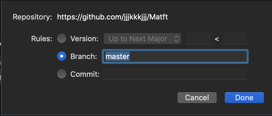
Project > Build Setting > +

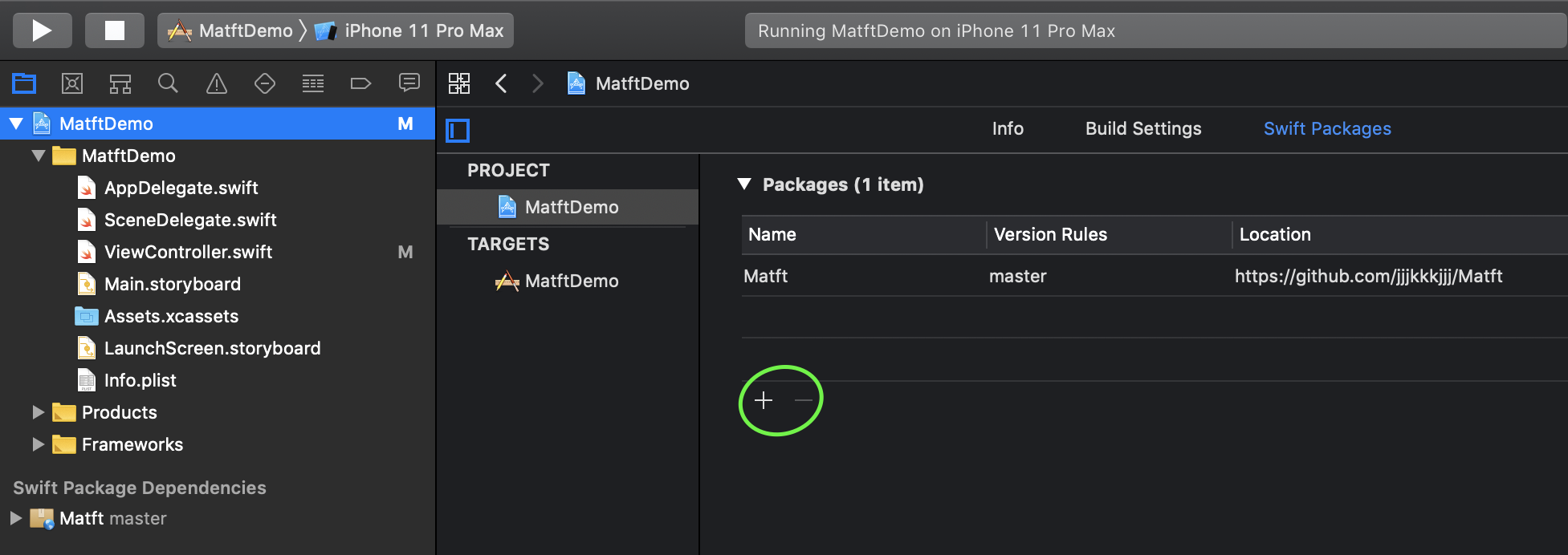
適宜選択

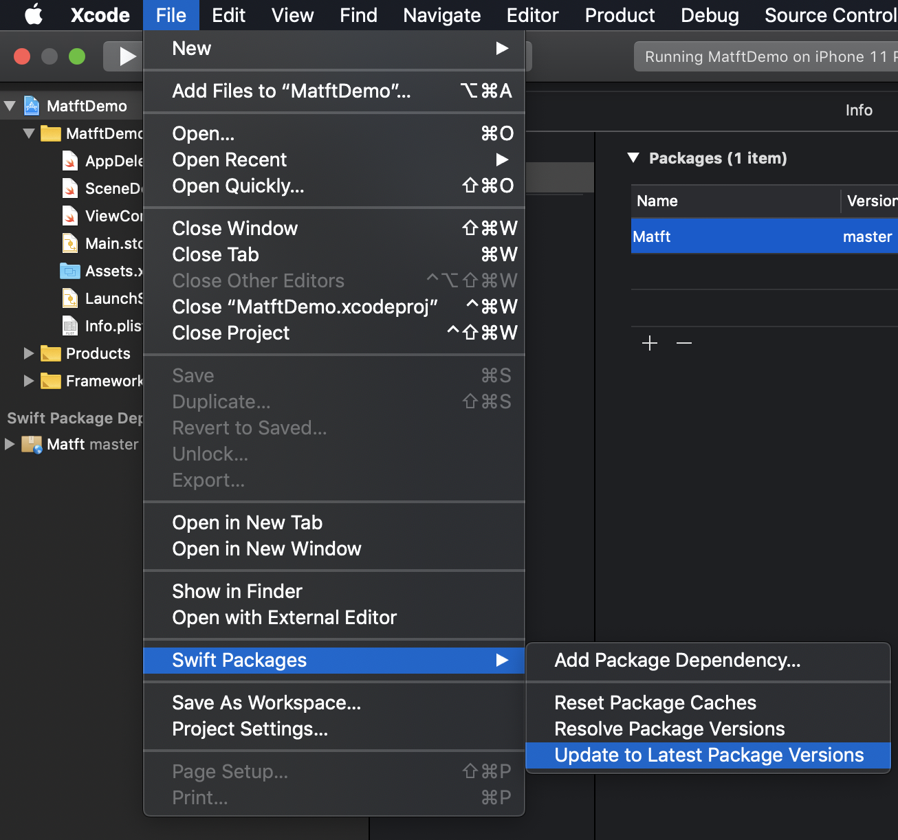
アップデート

File >Swift Packages >Update to Latest Package versions

CocoaPods

Podfile作成 (すでにある場合は無視)
  pod init
pod 'Matft'をPodfileに追記
  target 'your project' do
    pod 'Matft'
  end
インストール
  pod install
Performance

Accelerateに任せているので，計算は担保されていると言いましたが，足し算だけ速度を計算してみました．
時間があれば他の関数も調べます．．．

case Matft Numpy

1 1.14ms 962 µs

2 4.20ms 5.68 ms

3 4.17ms 3.92 ms

Matft
func testPefAdd1() {
        do{
            let a = Matft.mfarray.arange(start: 0, to: 10*10*10*10*10*10, by: 1, shape: [10,10,10,10,10,10])
            let b = Matft.mfarray.arange(start: 0, to: -10*10*10*10*10*10, by: -1, shape: [10,10,10,10,10,10])

            self.measure {
                let _ = a+b
            }
            /*
             '-[MatftTests.ArithmeticPefTests testPefAdd1]' measured [Time, seconds] average: 0.001, relative standard deviation: 23.418%, values: [0.001707, 0.001141, 0.000999, 0.000969, 0.001029, 0.000979, 0.001031, 0.000986, 0.000963, 0.001631]
            1.14ms
             */
        }
    }

    func testPefAdd2(){
        do{
            let a = Matft.mfarray.arange(start: 0, to: 10*10*10*10*10*10, by: 1, shape: [10,10,10,10,10,10])
            let b = a.transpose(axes: [0,3,4,2,1,5])
            let c = a.T

            self.measure {
                let _ = b+c
            }
            /*
             '-[MatftTests.ArithmeticPefTests testPefAdd2]' measured [Time, seconds] average: 0.004, relative standard deviation: 5.842%, values: [0.004680, 0.003993, 0.004159, 0.004564, 0.003955, 0.004200, 0.003998, 0.004317, 0.003919, 0.004248]
            4.20ms
             */
        }
    }

    func testPefAdd3(){
        do{
            let a = Matft.mfarray.arange(start: 0, to: 10*10*10*10*10*10, by: 1, shape: [10,10,10,10,10,10])
            let b = a.transpose(axes: [1,2,3,4,5,0])
            let c = a.T

            self.measure {
                let _ = b+c
            }
            /*
             '-[MatftTests.ArithmeticPefTests testPefAdd3]' measured [Time, seconds] average: 0.004, relative standard deviation: 16.815%, values: [0.004906, 0.003785, 0.003702, 0.005981, 0.004261, 0.003665, 0.004083, 0.003654, 0.003836, 0.003874]
            4.17ms
             */
        }
}
Numpy
In [1]:
import numpy as np
#import timeit

a = np.arange(10**6).reshape((10,10,10,10,10,10))
b = np.arange(0, -10**6, -1).reshape((10,10,10,10,10,10))

#timeit.timeit("b+c", repeat=10, globals=globals())
%timeit -n 10 a+b
962 µs ± 273 µs per loop (mean ± std. dev. of 7 runs, 10 loops each)
In [2]:
a = np.arange(10**6).reshape((10,10,10,10,10,10))
b = a.transpose((0,3,4,2,1,5))
c = a.T
#timeit.timeit("b+c", repeat=10, globals=globals())
%timeit -n 10 b+c
5.68 ms ± 1.45 ms per loop (mean ± std. dev. of 7 runs, 10 loops each)
In [3]:
a = np.arange(10**6).reshape((10,10,10,10,10,10))
b = a.transpose((1,2,3,4,5,0))
c = a.T
#timeit.timeit("b+c", repeat=10, globals=globals())
%timeit -n 10 b+c
3.92 ms ± 897 µs per loop (mean ± std. dev. of 7 runs, 10 loops each)
個人的に気に入っているところ

名前

複数型対応

Numpyぽさ

最後に

気まぐれで作成しましたが，思ったよりいい感じのものができました．ただただ僕の検索力不足なだけで，より良いライブラリがあるかもしれませんが，是非試していただけると嬉しいです．（環境依存のチェックができていませんので，是非お願いします．．．）
とにもかくにもいい勉強になりました．ありがとうございました．

参考

numpy
scipy
Accelerate
SwiftでNDArray書く（テストケースを参考にさせていただきました．）

Matft	Numpy
Matft.mfarray.shallowcopy	numpy.copy
Matft.mfarray.deepcopy	copy.deepcopy
Matft.mfarray.nums	numpy.ones * N
Matft.mfarray.arange	numpy.arange
Matft.mfarray.eye	numpy.eye
Matft.mfarray.diag	numpy.diag
Matft.mfarray.vstack	numpy.vstack
Matft.mfarray.hstack	numpy.hstack
Matft.mfarray.concatenate	numpy.concatenate

Matft	Numpy
Matft.mfarray.astype	numpy.astype
Matft.mfarray.transpose	numpy.transpose
Matft.mfarray.expand_dims	numpy.expand_dims
Matft.mfarray.squeeze	numpy.squeeze
Matft.mfarray.broadcast_to	numpy.broadcast_to
Matft.mfarray.conv_order	numpy.ascontiguousarray
Matft.mfarray.flatten	numpy.flatten
Matft.mfarray.flip	numpy.flip
Matft.mfarray.swapaxes	numpy.swapaxes
Matft.mfarray.moveaxis	numpy.moveaxis
Matft.mfarray.sort	numpy.sort
Matft.mfarray.argsort	numpy.argsort

Matft	Numpy
Matft.mfarray.file.loadtxt	numpy.loadtxt
Matft.mfarray.file.genfromtxt	numpy.genfromtxt

Matft	Numpy
Matft.mfarray.add	numpy.add
Matft.mfarray.sub	numpy.sub
Matft.mfarray.div	numpy.div
Matft.mfarray.mul	numpy.multiply
Matft.mfarray.inner	numpy.inner
Matft.mfarray.cross	numpy.cross
Matft.mfarray.equal	numpy.equal
Matft.mfarray.allEqual	numpy.array_equal
Matft.mfarray.neg	numpy.negative

Matft	Numpy
Matft.mfarray.math.sin	numpy.sin
Matft.mfarray.math.asin	numpy.asin
Matft.mfarray.math.sinh	numpy.sinh
Matft.mfarray.math.asinh	numpy.asinh
Matft.mfarray.math.sin	numpy.cos
Matft.mfarray.math.acos	numpy.acos
Matft.mfarray.math.cosh	numpy.cosh
Matft.mfarray.math.acosh	numpy.acosh
Matft.mfarray.math.tan	numpy.tan
Matft.mfarray.math.atan	numpy.atan
Matft.mfarray.math.tanh	numpy.tanh
Matft.mfarray.math.atanh	numpy.atanh

Matft	Numpy
Matft.mfarray.stats.mean	numpy.mean
Matft.mfarray.math.max	numpy.max
Matft.mfarray.math.argmax	numpy.argmax
Matft.mfarray.math.min	numpy.min
Matft.mfarray.math.argmin	numpy.argmin
Matft.mfarray.math.sum	numpy.sum

Matft	Numpy
Matft.mfarray.linalg.solve	numpy.linalg.solve
Matft.mfarray.linalg.inv	numpy.linalg.inv
Matft.mfarray.linalg.det	numpy.linalg.det
Matft.mfarray.linalg.eigen	numpy.linalg.eig
Matft.mfarray.linalg.svd	numpy.linalg.svd
Matft.mfarray.linalg.polar_left	scipy.linalg.polar
Matft.mfarray.linalg.polar_right	scipy.linalg.polar

case	Matft	Numpy
1	1.14ms	962 µs
2	4.20ms	5.68 ms
3	4.17ms	3.92 ms

　 Tweet
Qiitaで続きを読む

投稿日：2020-05-15T23:51:32+09:00

SwiftでN次元行列演算ライブラリMatftを作ってみた

はじめに

初投稿です．
タイトルの通りなのですが，SwiftでN次元行列演算ライブラリMatftを作ってみました．(Mat rix演算をする・Swi ftで，の略でMatftです笑)

事の発端は，会社の先輩の「Swiftで３行３列の逆行列を求めるコードを書いてほしい」という一言でした．
SwiftにはPythonのNumpyのようなN次元行列演算ライブラリがあるだろうと思ったのですが，調べると意外にもないんですよね．．．
公式のAccelerateは使い勝手悪そうだし，有名らしいsurgeも２次元まで？みたいでした．そんなこんなで，せっかくなので自作のN次元行列演算ライブラリを作ってみようと思いました．（３行３列の逆行列を求めるコードに対して，完全にオーバースペックですが笑）

さらにそんなこんなで，Matftができました．そしてせっかくなので共有してみようということで，現在に至ります．

概要

基本的にはPythonのNumpyにならって作成したので，関数名や使い方はNumpyとほぼ同じです．

宣言

宣言はndarrayなるMfArrayで多次元配列を生成します．
let a = MfArray([[[ -8,  -7,  -6,  -5],
                  [ -4,  -3,  -2,  -1]],

                 [[ 0,  1,  2,  3],
                  [ 4,  5,  6,  7]]])
print(a)
/*
mfarray = 
[[[ -8.0,       -7.0,       -6.0,       -5.0],
[   -4.0,       -3.0,       -2.0,       -1.0]],

[[  0.0,        1.0,        2.0,        3.0],
[   4.0,        5.0,        6.0,        7.0]]], type=Float, shape=[2, 2, 4]
*/
型

いろいろな型に対応させたかったので，それなりの型を用意しました．dtypeならぬMfTypeです．
let a = MfArray([[[ -8,  -7,  -6,  -5],
                  [ -4,  -3,  -2,  -1]],

                 [[ 0,  1,  2,  3],
                  [ 4,  5,  6,  7]]], mftype: .Float)
print(a)
/*
mfarray = 
[[[ -8.0,       -7.0,       -6.0,       -5.0],
[   -4.0,       -3.0,       -2.0,       -1.0]],

[[  0.0,        1.0,        2.0,        3.0],
[   4.0,        5.0,        6.0,        7.0]]], type=Float, shape=[2, 2, 4]
*/
let aa = MfArray([[[ -8,  -7,  -6,  -5],
                  [ -4,  -3,  -2,  -1]],

                 [[ 0,  1,  2,  3],
                  [ 4,  5,  6,  7]]], mftype: .UInt)
print(aa)
/*
mfarray = 
[[[ 4294967288,     4294967289,     4294967290,     4294967291],
[   4294967292,     4294967293,     4294967294,     4294967295]],

[[  0,      1,      2,      3],
[   4,      5,      6,      7]]], type=UInt, shape=[2, 2, 4]
*/
//Above output is same as numpy!
/*
>>> np.arange(-8, 8, dtype=np.uint32).reshape(2,2,4)
array([[[4294967288, 4294967289, 4294967290, 4294967291],
        [4294967292, 4294967293, 4294967294, 4294967295]],

       [[         0,          1,          2,          3],
        [         4,          5,          6,          7]]], dtype=uint32)
型一覧は以下のEnum型で定義しました．
※実を言うと，裏ではFloatかDoubleで保存しているので，UIntなんかは値が大きいとオーバーフローします．ただ，実用上は問題ないと思います．
 public enum MfType: Int{
    case None // Unsupportted
    case Bool
    case UInt8
    case UInt16
    case UInt32
    case UInt64
    case UInt
    case Int8
    case Int16
    case Int32
    case Int64
    case Int
    case Float
    case Double
    case Object // Unsupported
}
Indexing

Numpyでいうa[:, ::-1]のようなスライスも~で実装しました．
-1のような負のインデックスも実装しました．（これが一番苦労したかもしれません．．．）
let a = Matft.mfarray.arange(start: 0, to: 27, by: 1, shape: [3,3,3])
print(a)
/*
mfarray = 
[[[ 0,      1,      2],
[   3,      4,      5],
[   6,      7,      8]],

[[  9,      10,     11],
[   12,     13,     14],
[   15,     16,     17]],

[[  18,     19,     20],
[   21,     22,     23],
[   24,     25,     26]]], type=Int, shape=[3, 3, 3]
*/
print(a[2,1,0])
// 21
print(a[1~3]) //same as a[1:3] for numpy
/*
mfarray = 
[[[ 9,      10,     11],
[   12,     13,     14],
[   15,     16,     17]],

[[  18,     19,     20],
[   21,     22,     23],
[   24,     25,     26]]], type=Int, shape=[2, 3, 3]
*/
print(a[-1~-3])
/*
mfarray = 
    [], type=Int, shape=[0, 3, 3]
*/
print(a[~~-1])
/*
mfarray = 
[[[ 18,     19,     20],
[   21,     22,     23],
[   24,     25,     26]],

[[  9,      10,     11],
[   12,     13,     14],
[   15,     16,     17]],

[[  0,      1,      2],
[   3,      4,      5],
[   6,      7,      8]]], type=Int, shape=[3, 3, 3]*/
その他関数一覧

ここからは，具体的な関数一覧です．主な計算はAccelerateに任せているので，計算時間はある程度担保されていると思います．

生成系

Matft Numpy

Matft.mfarray.shallowcopy numpy.copy

Matft.mfarray.deepcopy copy.deepcopy

Matft.mfarray.nums numpy.ones * N

Matft.mfarray.arange numpy.arange

Matft.mfarray.eye numpy.eye

Matft.mfarray.diag numpy.diag

Matft.mfarray.vstack numpy.vstack

Matft.mfarray.hstack numpy.hstack

Matft.mfarray.concatenate numpy.concatenate

変換系

Matft Numpy

Matft.mfarray.astype numpy.astype

Matft.mfarray.transpose numpy.transpose

Matft.mfarray.expand_dims numpy.expand_dims

Matft.mfarray.squeeze numpy.squeeze

Matft.mfarray.broadcast_to numpy.broadcast_to

Matft.mfarray.conv_order numpy.ascontiguousarray

Matft.mfarray.flatten numpy.flatten

Matft.mfarray.flip numpy.flip

Matft.mfarray.swapaxes numpy.swapaxes

Matft.mfarray.moveaxis numpy.moveaxis

Matft.mfarray.sort numpy.sort

Matft.mfarray.argsort numpy.argsort

ファイル関係 saveが未完成です．

Matft Numpy

Matft.mfarray.file.loadtxt numpy.loadtxt

Matft.mfarray.file.genfromtxt numpy.genfromtxt

演算系

Matft Numpy

Matft.mfarray.add numpy.add

Matft.mfarray.sub numpy.sub

Matft.mfarray.div numpy.div

Matft.mfarray.mul numpy.multiply

Matft.mfarray.inner numpy.inner

Matft.mfarray.cross numpy.cross

Matft.mfarray.equal numpy.equal

Matft.mfarray.allEqual numpy.array_equal

Matft.mfarray.neg numpy.negative

初等関数系

Matft Numpy

Matft.mfarray.math.sin numpy.sin

Matft.mfarray.math.asin numpy.asin

Matft.mfarray.math.sinh numpy.sinh

Matft.mfarray.math.asinh numpy.asinh

Matft.mfarray.math.sin numpy.cos

Matft.mfarray.math.acos numpy.acos

Matft.mfarray.math.cosh numpy.cosh

Matft.mfarray.math.acosh numpy.acosh

Matft.mfarray.math.tan numpy.tan

Matft.mfarray.math.atan numpy.atan

Matft.mfarray.math.tanh numpy.tanh

Matft.mfarray.math.atanh numpy.atanh

面倒なので，省略します．．．笑
ここを見てください

高階関数系

Matft Numpy

Matft.mfarray.stats.mean numpy.mean

Matft.mfarray.stats.max numpy.max

Matft.mfarray.stats.argmax numpy.argmax

Matft.mfarray.stats.min numpy.min

Matft.mfarray.stats.argmin numpy.argmin

Matft.mfarray.stats.sum numpy.sum

線形代数系

Matft Numpy

Matft.mfarray.linalg.solve numpy.linalg.solve

Matft.mfarray.linalg.inv numpy.linalg.inv

Matft.mfarray.linalg.det numpy.linalg.det

Matft.mfarray.linalg.eigen numpy.linalg.eig

Matft.mfarray.linalg.svd numpy.linalg.svd

Matft.mfarray.linalg.polar_left scipy.linalg.polar

Matft.mfarray.linalg.polar_right scipy.linalg.polar

インストール

SwiftPMとCocoaPodに対応しました．

SwiftPM

Import

Project > Build Setting > +

適宜選択

アップデート

File >Swift Packages >Update to Latest Package versions

CocoaPods

Podfile作成 (すでにある場合は無視)
  pod init
pod 'Matft'をPodfileに追記
  target 'your project' do
    pod 'Matft'
  end
インストール
  pod install
Performance

Accelerateに任せているので，計算は担保されていると言いましたが，足し算だけ速度を計算してみました．
時間があれば他の関数も調べます．．．

case Matft Numpy

1 1.14ms 962 µs

2 4.20ms 5.68 ms

3 4.17ms 3.92 ms

Matft
func testPefAdd1() {
        do{
            let a = Matft.mfarray.arange(start: 0, to: 10*10*10*10*10*10, by: 1, shape: [10,10,10,10,10,10])
            let b = Matft.mfarray.arange(start: 0, to: -10*10*10*10*10*10, by: -1, shape: [10,10,10,10,10,10])

            self.measure {
                let _ = a+b
            }
            /*
             '-[MatftTests.ArithmeticPefTests testPefAdd1]' measured [Time, seconds] average: 0.001, relative standard deviation: 23.418%, values: [0.001707, 0.001141, 0.000999, 0.000969, 0.001029, 0.000979, 0.001031, 0.000986, 0.000963, 0.001631]
            1.14ms
             */
        }
    }

    func testPefAdd2(){
        do{
            let a = Matft.mfarray.arange(start: 0, to: 10*10*10*10*10*10, by: 1, shape: [10,10,10,10,10,10])
            let b = a.transpose(axes: [0,3,4,2,1,5])
            let c = a.T

            self.measure {
                let _ = b+c
            }
            /*
             '-[MatftTests.ArithmeticPefTests testPefAdd2]' measured [Time, seconds] average: 0.004, relative standard deviation: 5.842%, values: [0.004680, 0.003993, 0.004159, 0.004564, 0.003955, 0.004200, 0.003998, 0.004317, 0.003919, 0.004248]
            4.20ms
             */
        }
    }

    func testPefAdd3(){
        do{
            let a = Matft.mfarray.arange(start: 0, to: 10*10*10*10*10*10, by: 1, shape: [10,10,10,10,10,10])
            let b = a.transpose(axes: [1,2,3,4,5,0])
            let c = a.T

            self.measure {
                let _ = b+c
            }
            /*
             '-[MatftTests.ArithmeticPefTests testPefAdd3]' measured [Time, seconds] average: 0.004, relative standard deviation: 16.815%, values: [0.004906, 0.003785, 0.003702, 0.005981, 0.004261, 0.003665, 0.004083, 0.003654, 0.003836, 0.003874]
            4.17ms
             */
        }
}
Numpy
In [1]:
import numpy as np
#import timeit

a = np.arange(10**6).reshape((10,10,10,10,10,10))
b = np.arange(0, -10**6, -1).reshape((10,10,10,10,10,10))

#timeit.timeit("b+c", repeat=10, globals=globals())
%timeit -n 10 a+b
962 µs ± 273 µs per loop (mean ± std. dev. of 7 runs, 10 loops each)
In [2]:
a = np.arange(10**6).reshape((10,10,10,10,10,10))
b = a.transpose((0,3,4,2,1,5))
c = a.T
#timeit.timeit("b+c", repeat=10, globals=globals())
%timeit -n 10 b+c
5.68 ms ± 1.45 ms per loop (mean ± std. dev. of 7 runs, 10 loops each)
In [3]:
a = np.arange(10**6).reshape((10,10,10,10,10,10))
b = a.transpose((1,2,3,4,5,0))
c = a.T
#timeit.timeit("b+c", repeat=10, globals=globals())
%timeit -n 10 b+c
3.92 ms ± 897 µs per loop (mean ± std. dev. of 7 runs, 10 loops each)
個人的に気に入っているところ

名前

複数型対応

Numpyぽさ

最後に

気まぐれで作成しましたが，思ったよりいい感じのものができました．ただただ僕の検索力不足なだけで，より良いライブラリがあるかもしれませんが，是非試していただけると嬉しいです．（環境依存のチェックができていませんので，是非お願いします．．．）
とにもかくにもいい勉強になりました．ありがとうございました．

参考

numpy
scipy
Accelerate
SwiftでNDArray書く（テストケースを参考にさせていただきました．）

Matft	Numpy
Matft.mfarray.shallowcopy	numpy.copy
Matft.mfarray.deepcopy	copy.deepcopy
Matft.mfarray.nums	numpy.ones * N
Matft.mfarray.arange	numpy.arange
Matft.mfarray.eye	numpy.eye
Matft.mfarray.diag	numpy.diag
Matft.mfarray.vstack	numpy.vstack
Matft.mfarray.hstack	numpy.hstack
Matft.mfarray.concatenate	numpy.concatenate

Matft	Numpy
Matft.mfarray.astype	numpy.astype
Matft.mfarray.transpose	numpy.transpose
Matft.mfarray.expand_dims	numpy.expand_dims
Matft.mfarray.squeeze	numpy.squeeze
Matft.mfarray.broadcast_to	numpy.broadcast_to
Matft.mfarray.conv_order	numpy.ascontiguousarray
Matft.mfarray.flatten	numpy.flatten
Matft.mfarray.flip	numpy.flip
Matft.mfarray.swapaxes	numpy.swapaxes
Matft.mfarray.moveaxis	numpy.moveaxis
Matft.mfarray.sort	numpy.sort
Matft.mfarray.argsort	numpy.argsort

Matft	Numpy
Matft.mfarray.file.loadtxt	numpy.loadtxt
Matft.mfarray.file.genfromtxt	numpy.genfromtxt

Matft	Numpy
Matft.mfarray.add	numpy.add
Matft.mfarray.sub	numpy.sub
Matft.mfarray.div	numpy.div
Matft.mfarray.mul	numpy.multiply
Matft.mfarray.inner	numpy.inner
Matft.mfarray.cross	numpy.cross
Matft.mfarray.equal	numpy.equal
Matft.mfarray.allEqual	numpy.array_equal
Matft.mfarray.neg	numpy.negative

Matft	Numpy
Matft.mfarray.math.sin	numpy.sin
Matft.mfarray.math.asin	numpy.asin
Matft.mfarray.math.sinh	numpy.sinh
Matft.mfarray.math.asinh	numpy.asinh
Matft.mfarray.math.sin	numpy.cos
Matft.mfarray.math.acos	numpy.acos
Matft.mfarray.math.cosh	numpy.cosh
Matft.mfarray.math.acosh	numpy.acosh
Matft.mfarray.math.tan	numpy.tan
Matft.mfarray.math.atan	numpy.atan
Matft.mfarray.math.tanh	numpy.tanh
Matft.mfarray.math.atanh	numpy.atanh

Matft	Numpy
Matft.mfarray.stats.mean	numpy.mean
Matft.mfarray.stats.max	numpy.max
Matft.mfarray.stats.argmax	numpy.argmax
Matft.mfarray.stats.min	numpy.min
Matft.mfarray.stats.argmin	numpy.argmin
Matft.mfarray.stats.sum	numpy.sum

Matft	Numpy
Matft.mfarray.linalg.solve	numpy.linalg.solve
Matft.mfarray.linalg.inv	numpy.linalg.inv
Matft.mfarray.linalg.det	numpy.linalg.det
Matft.mfarray.linalg.eigen	numpy.linalg.eig
Matft.mfarray.linalg.svd	numpy.linalg.svd
Matft.mfarray.linalg.polar_left	scipy.linalg.polar
Matft.mfarray.linalg.polar_right	scipy.linalg.polar

case	Matft	Numpy
1	1.14ms	962 µs
2	4.20ms	5.68 ms
3	4.17ms	3.92 ms

　 Tweet
Qiitaで続きを読む

投稿日：2020-05-15T23:05:48+09:00

ゼロから始めるLeetCode Day26「94. Binary Tree Inorder Traversal」

概要

海外ではエンジニアの面接においてコーディングテストというものが行われるらしく、多くの場合、特定の関数やクラスをお題に沿って実装するという物がメインである。

その対策としてLeetCodeなるサイトで対策を行うようだ。

早い話が本場でも行われているようなコーディングテストに耐えうるようなアルゴリズム力を鍛えるサイト。

せっかくだし人並みのアルゴリズム力くらいは持っておいた方がいいだろうということで不定期に問題を解いてその時に考えたやり方をメモ的に書いていこうかと思います。

Leetcode

ゼロから始めるLeetCode 目次

前回
ゼロから始めるLeetCode Day25「70. Climbing Stairs」

基本的にeasyのacceptanceが高い順から解いていこうかと思います。

Twitterやってます。

問題

543. Diameter of Binary Tree
難易度はeasy。
Top 100 Liked Questionsからの抜粋です。

二分木が与えられるので、その木の直径を返します。
なお、ここでの直径とは各ノード間の中で最も長い距離を行き来するような通路のことを指します。
Example:

Example:
Given a binary tree
          1
         / \
        2   3
       / \     
      4   5    
Return 3, which is the length of the path [4,2,1,3] or [5,2,1,3].

Note: The length of path between two nodes is represented by the number of edges between them.
この場合だと4から3までいく場合と5から3までいくものの二つが最長であり、間にある枝の数が3なので3を返します。

解法

深さ優先探索でときました。
# Definition for a binary tree node.
# class TreeNode:
#     def __init__(self, val=0, left=None, right=None):
#         self.val = val
#         self.left = left
#         self.right = right
class Solution:
    def diameterOfBinaryTree(self, root: TreeNode) -> int:
        self.ans = 0

        def dfs(node):
            if not node:
                return 0
            right = dfs(node.right)
            left = dfs(node.left)
            self.ans = max(self.ans,left+right)
            return max(left,right) + 1

        dfs(root)
        return self.ans
# Runtime: 44 ms, faster than 72.73% of Python3 online submissions for Diameter of Binary Tree.
# Memory Usage: 15.9 MB, less than 51.72% of Python3 online submissions for Diameter of Binary Tree.
基本的な流れは一般的な深さ優先探索のそれと一緒です。ただ、今回は長さを調べる必要があるので、そのための変数ansを用意し、計算を付け加えました。

割と過去の木の問題でも深さ優先探索ばかり書いているのでそろそろ幅優先探索とかも勉強しなきゃなぁと思います。
今日はもう遅いのでこれでお終いです、お疲れ様でした。

良さげな解答が他にあれば追記します。

　 Tweet
Qiitaで続きを読む

投稿日：2020-05-15T22:43:28+09:00

【数式なしの量子コンピュータ】　新視点セルオートマトンとグローバー　　２回目１、０ではない重ね合わせでの初期状態

連載記事の２回目　１，０ではない重ね合わせでの初期状態
いきなりこの回を読むと意味不明かもしれない。その場合は、１回目 を読んで頂きたい。本連載記事の目的と概要を投稿している。今回から具体的なBlueqatでの量子コンピュータの記事となる。ただ本題となるセルオートマトンの量子アルゴリズムやその時間発展は4回目以降の予定。今回の目玉は１，０ではない確率初期状態のセッティング方法とBlueqatで確率だの状態ベクトルだのをどう料理するのかである。まず、その前提としてq-camの構造とモジュールを紹介する。

2-1. q-camの構造とモジュール

Githubに公開したq-camsの中にあるプログラムとモジュールの表を示す。尚、以降、q-camsと表記した部分は、Githubのリポジトリ―にリンクしている。尚、御覧のとおりファイル名の拡張子はpy、つまり言語はpythonである。

ファイル名内容説明のある回

qcam.py q-cam専用の、初期確率セット
ベクトルと確率の抽出、出力、プロットなどのモジュール２回目

qmcn.py Blueqatで汎用的に使用できるモジュール
マルチ制御NOTゲート　CCCX～CCCCCCX
フレドキンゲート３回目

probshot.py セットした確率を観測でみる２回目

probvect.py セットした確率を状態ベクトルでみる２回目

q-cam30r.py ルール30　セルオートマトン４回目

q-cam60r.py ルール60　セルオートマトン４回目

q-cam90r.py ルール90　セルオートマトン４回目

q-cam102r.py ルール102　セルオートマトン４回目

q-cam110r.py ルール110　セルオートマトン４回目

q-cam184r.py ルール184　セルオートマトンルール５回目

q-cam184i.py ルール184　セルオートマトン虚数版５回目

q-cambbr.py ソリトン（箱玉系）セルオートマトン６回目

q-camgr.py グローバーアルゴリズム　７回目

q-camの構造と言っているのは上の表のq-cam30r.py以下のプログラムにおける共通構造のことである。今回紹介する「１，０ではない確率初期状態のセッティング方法」は、qcam.pyのモジュール内の関数であり、またBlueqatで確率だの状態ベクトルだのをどう料理するのかは、probshot.pyとprobvect.pyと言うプログラムを用いての説明となる。モジュールqcamとqmcnはプログラムと同じフォルダにダウンロードして使用することが前提。各、プログラムはコンソールから動かす。さて、q-camの構造は単純で以下の通りである。

①モジュールの読み込み部
②定数セット部
③Blueqatで記述した量子プログラム部(Q-process)
④メインの制御部
⑤終了部分（プロットなど）

順に実際のコード例で説明しよう。
①モジュールの読み込み部
example1.py
from blueqat import Circuit
import numpy as np
import qcam
import qmcn as q
一行目はBlueqatを使う場合、必要な読み込みで詳しくはこちらを参照。https://blueqat.readthedocs.io/ja/latest/
二行目は、numpyを使用するため。３行目のqcamは、q-camプログラムで必須のモジュール。
import qcam as qc　などとし略称でモジュールを使用できるようにしても、勿論OK。ラストの行にあるqmcnは、マルチ制御NOTゲートを使わない限りは不要で、q-camsのプログラム群の中ではグローバーアルゴリズムとソリントセルオートマトン以外では使用しない。

②定数セット部
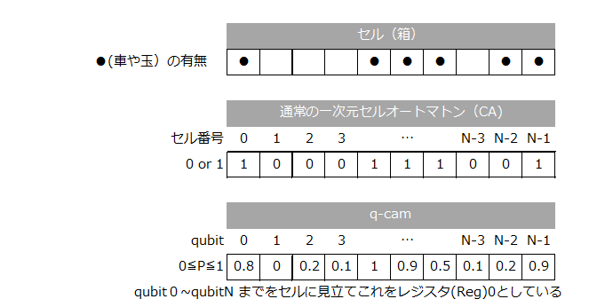
example2.py
N=10                            # number of cells
R=2                             # number of registers

# initial probability distribution
initial_a=np.array([0.8,0,0.2,0.1,1,0.9,0.5,0.1,0.2,0.9],dtype='float')
Nはセルオートマトンでのセル数（下図参照）、Rはレジスタ数で、この積NRが全量子ビット数となる。セルに見立てたN個の量子ビット(0～N-1)もレジスタに含まれ、これをレジスタ0とする。セル数Nはユーザーが好きに書き変えられるが、レジスタ数はセルオートマトンのアルゴリズムに依存する。詳しくは４回目に説明する。Blueqatの場合、量子ビット数の上限は32bitなので、NR≦32だが、24ぐらいを超えると計算時間が長くなる。また、配列initial_a は、まさに今回の「０，１ではない確率の集合」を現しており、左から順に、セルに割り当てらる。従ってこの配列の要素数は必ず、上記のセル数と一致しなければならない。下図参照。これらの確率を実際の量子ビットにセットするのが、１，０ではない確率初期状態のセッティング方法であって2-2で説明する。

上のコード内では省略したが定数セット部はさらにつづが、主として各レジスタのスタート量子ビット番号とラスト量子ビット番号の割り当てである。

③Blueqatで記述した量子プログラム部(Q-process)
この部分は、まさにBlueqatで量子アルゴリズムを記述する部分であり、内容は４回目に説明する。最も簡単な例として、ルール102の場合の量子プログラム部を示す。
example3.py
def qproc():
    for i in range(N):
        c.cx[1+i, i]
    return
④メインの制御部
メインの制御部の代表的例
example4.py
pstep=0
ret='y'

while ret=='y':

    pstep+=1

    c=Circuit(N)

    pinitial_a=probability_a    
    if pstep==1:
        pinitial_a=initial_a

    qcam.propinit(N,c,pinitial_a)
    qproc()
    master_a=np.array(c.run())

    num,vector_a,prob_a=qcam.qvextract(N,R,1,master_a)
    stdev,probability_a=qcam.qcalcd(N, num,vector_a,prob_a)
    qcam.qcresultout(N, pstep, num,pinitial_a,vector_a,prob_a,stdev,probability_a)

    stepdist_a[pstep,0:N]=probability_a[0:N]
    stdev_a[pstep]=stdev

    ret=input(' NEXT(Y/N)?')
pstepは時間発展（１回目参照）のカウンタで初期を０としている。配列pinitial_aはその時間ステップのセルオートマトンの遷移前の初期状態で、時刻1、つまりpstep=1のときは、initial_aそのものである。まずはじめにpinitial_a配列の確率を量子ビットにセットする。それが2-2で説明するqcamモジュール内のpropinit関数である。これでセル番号0～N-1に見立てたreg0の量子ビット番号0～N-1に確率（確率振幅）がセットされる。セット後、qproc()で遷移のためのBlueqatの量子プロセスとなる。実際の実行はBlueqatのc.run()である。このBlueqatの命令は2-3で説明する状態ベクトルを見る方法である。状態ベクトルといいつつ実はBlueqatではベクトルそのものがこれで分かるわけではなく、その状態ベクトルの確率振幅がベクトルの数だけ、複素数表記の一次元リストの形で戻ってくる。それをmaster_aという一次元の配列に取り込み、これから状態ベクトルだの、確率だのを抽出し、計算をする。

ある時刻ステップ（pstep）のセルの確率の結果は、次の時刻ステップ（pstep+1）の初期状態となるように代入している。stepdist_a[pstep,0:N]=probability_a[0:N] コンソール上で NEXT(Y/N)?と入力を促し、ｙと入力した場合は、次の時間ステップに進む。この繰り返しで、１ステップづつ時間発展をさせていく。ｙ以外を入力した場合は以下の⑤に続く。

⑤終了部分（プロットなど）
時間発展の結果をまとめて表示する関数qcam.qcfinalとセルオートマトンの時間発展を視覚的に表現するための関数qcam.qcamplotを実行し終了となる。尚、これらの出力内容に関しては４回目で詳述する。

2-2. 1,0ではない確率的初期状態（ry 又は rx 又は u3 ゲートで作る）

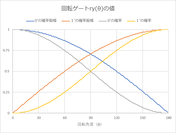
さて、いよいよ、セルに見立てた量子ビットに「０，１ではない確率の集合」をセットする方法である。ある量子ビット、ここではi番目の量子ビットをqubit[i]と表現しよう。またqubit[i] の状態を示すのを qubit[i]⇒ と表現しよう。確率ゼロをセットするのは簡単で、BlueqatのCircuitオブジェクトを作成後、何もしなければゼロ状態である。つまり qubit[i]⇒0 である。状態１をセットするのも簡単でBlueqatのXゲート(反転あるいはフリップゲートとも称する）を使えばqubit[i]⇒1となる。コードで記せば、x[qubit[i]]である。では、次に０と１がちょうど半々で重ねあった状態、つまり確率0.5、qubit[i]⇒0.5は？　これも簡単でアダマールゲートを使えば良い。コードで記せば、h[qubit[i]]である。では、qubit[i]⇒0.33とするには？

今、y軸での回転ゲートryで0度から180度まで１度おきに回転させた時の一つのqubitの状態１と状態０のもっている割合、つまり重ね合わせの混合割合の平方根（＝確率振幅）と、それを二乗した値＝混合割合＝確率を見てみよう。（グラフ）
参考コード
example5.py
from blueqat import Circuit
import numpy as np

for j in range(180):

    c=Circuit(1)
    theta=j*np.pi/180   
    c.ry(theta)[0]

    result=c.run()      

    q0=round(result[0].real,2)
    q1=round(result[1].real,2)
    q2=round(result[0].real**2,2)
    q3=round(result[1].real**2,2)

    print(j,'{0:>6} {1:>6} {2:>6} {3:>6}'.format(q0,q1,q2,q3)) 
セルに見立てたひとつの量子ビットにセットするのは、車や玉がそのセルにどの程度存在しているのか、つまり「１（車あるいは玉などが有）」の確率である。（100%そこに車が存在していれば１、全くいなければ0%だが、33%そこに車がいるとは？）グラフを見てわかる通りryの確率振幅は単なるsin関数（実際には$\sinθ/2$）である。その確率（確率振幅の二乗）は $\ P_1=sin^2θ/2$ 　である。従って、ある確率Pが与えられた場合、この式から角度θが逆算できる。数式が出て申し訳ないが、$\ θ=2arcsin ( \sqrt{P_1}\ ) $、このθをryゲートの回転角として量子ビットに適用すれば、その量子ビットに所望の確率（確率振幅）をセットすることができる。確率0.5、つまりアダマールの場合、θ＝π/2、つまり90度となる。尚、「１」はπ（180度）、「０」はゼロ度である。

qcamモジュールのpropinit関数に引数として、セル数N、Blueqatのサーキットオブジェクトc、セルに見立てた量子ビットの各々の確率の配列を渡すと、ryゲートを用いて確率をセットできる。
example6.py
def propinit(NN, c, ppinit_a):

    for i in range(NN):                 
        theta=2* np.arcsin(np.sqrt(ppinit_a[i]))    # Correlation between Probability and Rotation Angle
        c.ry(theta)[i]                      # You can change from ry to rx.     
    return
また、y軸での回転ゲートに代えてｘ軸での回転ゲートrxも全く同様に使用できる。（ryをrx書き換えるだけでOK)　rxに置き換えた場合、「０」はryの場合と全く同じだが、「１」には実数での確率振幅はなくなり、虚数の確率振幅を持つようになる。だが、二乗すれば虚数（複素数）でも確率となり同じである。それは兎に角「１」の確率 $P_1$は、「０」の余事象であるので、$P_1＝1-P_0$。また、$P_1$ は $P_1=cos^2θ/2$ であるため、$P_1＝1-cos^2θ/2=sin^2θ/2$ となる。故に、これはryゲートの場合と全く同様となる。
u3ゲートで確率＋αを与えてみた

一つの量子ビットに対して、重ね合わせ的には「１」とその余事象である「０」しかなく、確率としての「１」、「０」を捉えているが、確率振幅であれば、もう一つ情報を追加できると考えた。「１」の実数と虚数、「０」の実数部である。「０」の虚数部は常にゼロである。確率以外の情報を増やすと何が生じるのか知りたくて考えたのだが... 　当然、セルに見立てた量子ビットには単なる確率ではなくて、複素数をセットしなくてはならない。「１」の確率を $P_A$、 $P_B$の二つにわけ、前者を実数、後者を虚数に振り分けることとして、残りは余事象である、$P_0$とする。今、$P_0=0.3$とした場合、$P_A+P_B=0.7$。さらに$P_A=0.5$、$P_B=0.2$　とする場合、initial_aの配列要素としてnumpyのcomplex型を用いて、0.5+0.2j と記せばよい。これを量子ビットにセットするには、ユニバーサルゲートであるu3を使えばできる。u3のθ、φ、λをryやrxの時と同様に考えて以下の式を得る。
* $θ=2arccos\sqrt P_B$
* $φ＝arccos\sqrt{P_A/(1-P_0)}$
* $λ＝arcsin\sqrt{P_B/(1-P_0)}$
以下はqcam.impropinitのコードで、q-cam184iのみに使用される。
example7.py
def rotangle(probi):

    Areal=probi.real
    Bimag=probi.imag
    Zero=1-Areal-Bimag

    if Zero==1:
        phi=0
        lam=0
    else:
        phi=np.arccos(np.sqrt(Areal/(1-Zero)))
        lam=np.arcsin(np.sqrt(Bimag/(1-Zero)))

    theta=2*np.arccos(np.sqrt(Zero))

    return theta,phi,lam

def impropinit(NN, c, ppinit_a):

    for i in range(NN):                 
        ptheta,pphi,plam=rotangle(ppinit_a[i])      
        c.u3(ptheta,pphi,plam)[i]
    return
2-3. Blueqatの状態ベクトル表示からのベクトルと確率の抽出

Blueqatには、量子コンピューティングの結果をみる手段として、観測と状態ベクトルの「覗き見」が用意されている。観測に関しては後述。状態ベクトルののぞき見命令はc.run()である。状態ベクトルを見る方法ではあるが、ベクトルそのものがこれで分かるわけではなく、その状態ベクトルの確率振幅が状態ベクトルの数だけ、複素数表記の一次元リストの形で戻ってくる。状態ベクトルとその数って？　例えば、全部で４量子ビットなら、状態ベクトルは、００００、１０００、０１００、１１００、００１０、１０１０、０１１０、１１１０、０００１、１００１、０１０１、１１０１、００１１、１０１１、０１１１、１１１１の１６個である。状態ベクトルの数は $2^4=16$ 、つまり、全部でn量子ビットならば $2^n$ 個となる。q-camの場合の全量子ビット数は大概20を超えるので、$2^{20}=1,048,576$　つまり百万個以上である。

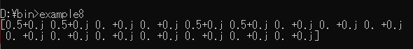
Blueqatで確率振幅が状態ベクトルの数だけ複素数表記の一次元リストの形で戻ってくるとは、要は百万個以上の複素数の要素を持ったリストが答えとなっているということである。だが、幸いq-cmaの場合、その大多数の状態ベクトルは確率振幅ゼロ、つまり意味なしである。だから、確率振幅なり、その二乗である確率（その状態ベクトルが出現する確率）がゼロより大きいものだけを抽出すればよい。それは、しらみつぶしに c.run() の戻り値リストの先頭から順に値がゼロより大のものを抽出するということである。しかし、複素数の値そのものは確率振幅であって、それがどの状態ベクトルの値なのかが分からないのでは。・・・んなわけはないはず。

上述した４量子ビット時の状態ベクトルを左が小さい桁で表した二進数表記と考えると左から順に大きくなっていく。１０進数に直せば、０，１，２，３，４，５，６，７，８，９，１０，１１，１２，１３，１４，１５である。Blueqatの状態ベクトルの覗き見の結果は、まさにこの順で出力されている。例えば、全４量子ビットで、０番目と２番目の量子ビットにアダマールゲートを適用した時のc.run() の結果を見てみよう。
example8.py
from blueqat import Circuit

c=Circuit(4)
c.h[0,2]    
print(c.run())
上のコードをコンソールで実行した結果が以下である。

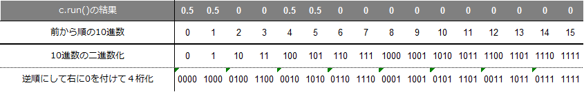
このc.run() の結果に、前から順番に１０進数を付けた後、それを二進数に変換し、さらに、その二進数を逆順にして、４桁に満たない場合は右に４桁になるように０をつける。（下表参照）これでできた二進数こそ、複素数のリストに対応した状態ベクトルである。

リストの先頭から１づつ増加するカウンタでループさせた場合、このカウンタこそが、確率振幅に対応した状態ベクトルである。前述したが、q-camでは状態ベクトルが百万以上になるため、確率振幅なり、その二乗である確率（その状態ベクトルが出現する確率）がゼロより大きいものだけを抽出し、その時のカウンタのみから状態ベクトルを求めれば良く、そのことを抽出と称している。その抽出関数がqcamモジュールのqcam.qvextractである。pythonで10進数のカウンタをbinで２進数化した時、先頭に二進数であることを明示する'0b'が付いてくる。この'0b'付き二進数をリスト化してdelで'0b'をカットする。さらに、qcamの場合、確率として必要なのは全量子ビット（NR個)の内、ゼロレジスタ（初めのN個）の部分のみであるため、全量子ビットのベクトルから一番末尾に来るN個分をスライスする。
example9.py
def qvextract(NN,RN,RW,extract_a):

    reg0_a=np.array([['0']*NN]*2**NN)                   # [result-number,cell-number]
    tempo_list=['0']*NN
    eprobv_a=np.array([0]*2**NN,dtype='complex')
    ereprov_a=np.array([0]*2**NN,dtype='float')

    nm=0
    for i in range(len(extract_a)):                                 
        if abs(extract_a[i])>0.0001:                # Decimal 'i' is the very vector!           
            tempo1_list=list(bin(i))                # vector extraction but reversed. (Decimal to Binary)
            del tempo1_list[0:2]                    # Delete '0','b' in tempo list                  
            tempo1_list[0:0]=['0']*(NN*RN-len(tempo1_list))     # Zero-fill to adjust digits

            reg0_a[nm,0:NN]=tempo1_list[(1-RW)*NN-1:-RW*NN-1:-1]    # slice and reverse 
            eprobv_a[nm]=extract_a[i]               # Probability amplitude
            nm+=1

    for i in range(nm):             
        ereprov_a[i]=eprobv_a[i].real*eprobv_a[i].real+eprobv_a[i].imag*eprobv_a[i].imag

    return nm,reg0_a,ereprov_a
2-4.　Blueqatのベクトルと観測

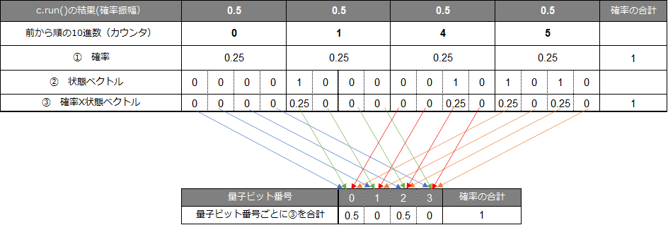
2-3.までで c.run()の結果から状態ベクトルとそれに対応したそのベクトルが出現する確率までが抽出できた。だが、知りたいのは量子ビットごとの「１（車あるいは玉などが有）」の確率である。2-3.での例では、０番目と２番目の量子ビットにアダマールゲートを適用した。ということは、2-2.で説明した「０と１がちょうど半々で重ねあった状態、つまり確率0.5」を０番目と２番目の量子ビットにセットしたことを意味している。つまり、qubit[0]⇒0.5　qubit[2]⇒0.5となっている筈である。

2-3.の結果の中から確率振幅>0のものだけを抽出すると、１０進数で言う０，１，４，５である。これらの状態ベクトルは下表に示した通りである。今、確率①（確率振幅の二乗）とベクトルの各要素②との積を③とする。各ベクトルごとのこの③の値を、量子ビット番号ごとに和をとると、表に示した通り、０番目と２番目の量子ビットが0.5となる。つまり、qubit[0]⇒0.5　qubit[2]⇒0.5であり、これでやっと c.run()の結果から知りたいことを知ることができた。

q-camで、この処理を行う関数が以下のqcam.qcalcdである。二次元配列 csum_a に、j番目のベクトルのi番目の量子ビットの値③を格納する。こうすることによりループを回さずにnumpyのsum関数np.sum(csum_a,axis=0)を用いて、量子ビットごとの確率を求め、それを一次元配列cproreal_aに格納している。こうすることにより、c.run()と言うBlueqatの「覗き見」命令から量子ビットごとの「１（車あるいは玉などが有）」の正確な確率を得ることができる。
example10.py
def qcalcd(NN, cnum, cvect_a, cprobare_a):

    cproreal_a=np.array([0]*NN,dtype = 'float')     
    csum_a=np.array([[0]*NN]*cnum,dtype = 'float')

    for j in range(cnum):
        for i in range(NN):
            csum_a[j,i]=float(cvect_a[j,i])*cprobare_a[j]

    cproreal_a=np.sum(csum_a,axis=0)

    cstd=np.std(cproreal_a)

    return cstd,cproreal_a
だが、リアルの量子コンピュータでは「覗き見」などできないはずである。代わりに「観測」を行う。この「観測」を行ってしまうと、残念なことに、ある量子ビットが１と０を同時にある割合で重ね合わされていたとしても、その割合を直接的に知ることはできず、「観測」をしたとたんに、結果は１か０のどちらかになってしまう。この量子力学上の残念な性質を波束の収縮と言う。でも心配することはない。同じ試行（この場合は量子コンピューティング）を何度も繰り返すと、１状態が出る回数と０状態が出る回数の割合を知ることができる。例えば、１００回繰り返して、１状態が６０回、０状態が４０回という結果であれば、大体、状態１の確率が0.6であると知ることができる。

Blueqatではこのような観測と試行の繰り替えしとして、 c.m[:].run(shots=number) （numberは試行回数）が準備されている。下のプログラムprobshot.pyではセル数を８とし、試行回数を1000回としている。0~N-1量子ビットの初期セット確率は [0.4,0,1,0.5,1,0,0,0.2] とした。これらは自由に書き換えて実行することができる。量子ビットにこの確率セットした後、何の量子コンピューティングもせずに観測のみ実行する。何の量子コンピューティングもせずに観測しているので、当然セットした確率と同じ確率が結果となるはずであるが・・・

尚、c.m[:].run(shots=number)の結果はdict（辞書）型で、キーは状態ベクトル、値はその状態ベクトルが出現した回数である。従って、この出現回数を試行回数で割れば確率となる。
コード
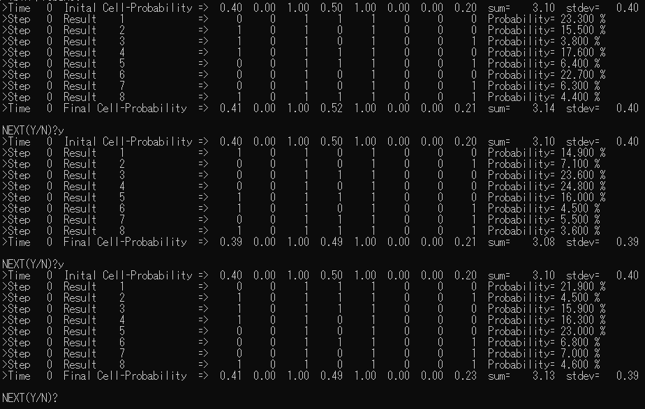
probshot.py
from blueqat import Circuit
import numpy as np
import qcam

# -------- Setting ------------------------------------------------------------------

N=8                                 # number of qubits :You can change.
nrun=1000                           # number of runs :You can change.
initial_a=np.array([0.4,0,1,0.5,1,0,0,0.2],dtype='float')       # initial probability distribution :You can change.
vector_a=np.array([[0]*N]*(2^N),dtype='int')
csum_a=np.array([[0]*N]*(2^N),dtype='float')
final_a=np.array([0]*N,dtype='float')
prob_a=np.array([0]*(2^N),dtype='float')


#---------- Main Body ----------------------------------------------------------------

ret='y'
while ret=='y':

    c=Circuit(N)
    qcam.propinit(N,c,initial_a)

    ans=c.m[:].run(shots=nrun)
    num=len(ans)
    kk=list(ans.keys())
    vv=list(ans.values())

    for i in range(num):
        vector_a[i,0:N]=list(kk[i])             # Result Vectors
        prob_a[i]=vv[i]/nrun

    stdev,final_a=qcam.qcalcd(N,num,vector_a, prob_a)
    qcam.qcresultout(N, 0, num, initial_a, vector_a, prob_a,stdev, final_a)

    ret=input(' NEXT(Y/N)?')
以下、コンソールでの実行結果である。NEXT(Y/N)?でｙを入力すると、q-camのような時間発展ではなく、ただ単に同じことを繰り返す。

この出力結果の見方を簡単に説明する。TimeとStepはq-camの用の時間発展を示しているのでここでは無視。sumは各量子ビットの確率の単純な和。またstdevはその分散だが、やはりここでは関係ない。Initial Cell-Probability は初期にセットした確率。Result 1 からは確率が0より大きい結果となった状態ベクトルとそのベクトルの確率（＝出現回数／試行回数の％）をProbabilityとして出力している。最後の Final Cell-Probability は状態ベクトルとその確率から計算した、各量子ビットごとの確率である。
さて、当然、何も処理をしていないのだから Initial Cell-Probability と Final Cell-Probability　は等しくなければならないが、どうであろう。１０００回の試行を三度繰り返しているが、小数点第２位では結構な誤差が出てしまっている上、毎回少しずつ異なる。観測とは、あるいは波束の収縮とは、このようなものだと理解するしかない。（この観測もリアル量子コンピュータではなく、それらしくシミュレートしたものであることは言うまでもない）

q-cmaでは正確な解が欲しい。となると、c.run()での覗き見を使うしかない。量子コンピュータと謳いながら・・・。シミュレーターさまさまである。念のために確認してみよう。
コード
probvect.py
from blueqat import Circuit
import numpy as np
import qcam

# -------- Setting ------------------------------------------------------------------

N=8                                 # number of cells :You can change.
R=1                                 # number of registries      
initial_a=np.array([0.4,0,1,0.5,1,0,0,0.2],dtype='float')           # initial probability distribution :You can change.
vector_a=np.array([[0]*N]*(2^N),dtype='int')
csum_a=np.array([[0]*N]*(2^N),dtype='float')
final_a=np.array([0]*N,dtype='float')

#---------- Main Body ----------------------------------------------------------------

ret='y'
while ret=='y':

    c=Circuit(N)
    qcam.propinit(N,c,initial_a)

    master_a=np.array(c.run())

    num,vector_a,prob_a=qcam.qvextract(N,R,1,master_a)
    stdev,final_a=qcam.qcalcd(N, num,vector_a,prob_a)
    qcam.qcresultout(N, 0, num, initial_a, vector_a, prob_a,stdev, final_a)

    ret=input(' NEXT(Y/N)?')
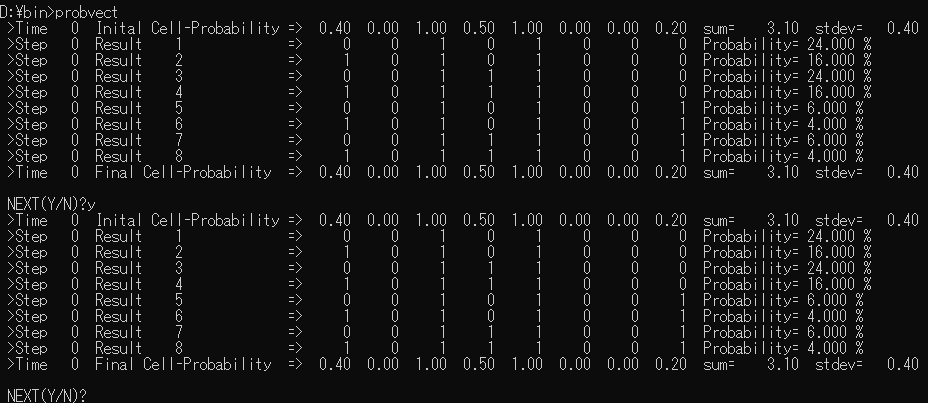
以下、コンソールでの実行結果である。

当たり前のことだが、Initial Cell-Probability と Final Cell-Probability　は完全に一致する。

第二回目のサマリー

１台の量子コンピュータで１０００回繰り返し観測するのと、１回だけ１０００台の量子コンピュータで観測するのと、同じ結果になるのか？エルゴート的には同じなんだろう。でも確率って、当たるも八卦当たらぬも八卦。次回、三回目は、がらっと変わって制御制御制御制御制御制御・・・ゲートの実装。

ファイル名	内容	説明のある回
qcam.py	q-cam専用の、初期確率セットベクトルと確率の抽出、出力、プロットなどのモジュール	２回目
qmcn.py	Blueqatで汎用的に使用できるモジュールマルチ制御NOTゲート　CCCX～CCCCCCX フレドキンゲート	３回目
probshot.py	セットした確率を観測でみる	２回目
probvect.py	セットした確率を状態ベクトルでみる	２回目
q-cam30r.py	ルール30　セルオートマトン	４回目
q-cam60r.py	ルール60　セルオートマトン	４回目
q-cam90r.py	ルール90　セルオートマトン	４回目
q-cam102r.py	ルール102　セルオートマトン	４回目
q-cam110r.py	ルール110　セルオートマトン	４回目
q-cam184r.py	ルール184　セルオートマトンルール	５回目
q-cam184i.py	ルール184　セルオートマトン虚数版	５回目
q-cambbr.py	ソリトン（箱玉系）セルオートマトン	６回目
q-camgr.py	グローバーアルゴリズム	７回目

　 Tweet
Qiitaで続きを読む

投稿日：2020-05-15T21:58:35+09:00

SwitchBot温湿度計の値をRaspberryPiでロギング

はじめに

本記事は、Omron環境センサ（BAG型）の記事と同内容を、
低価格で画面表示付きのSwitchBot温湿度センサで実施した記事です。

SwitchBotとは？

中国・深圳のメーカーWonderlabs Inc.が開発した、家庭用IoT機器シリーズです。
今回は、上記シリーズの温湿度センサ

を使用します。
低価格（2000円くらい）でスマホアプリやAPIでのデータ取得、画面表示まで揃った多機能が魅力です。

必要なもの

・RaspberryPi（今回はPi3Model Bを使用）
・Python実行環境（今回はpyenvでPython3.7.6使用）
・SwitchBot温湿度センサ

手順

①RaspberryPiとセンサのBluetooth接続確認
②センサの測定値をPythonで取得
③PythonからGASのAPIを叩いてスプレッドシートにデータ書き込み
④スクリプトの定期実行

こちらを参考にさせて頂きました。
https://qiita.com/warpzone/items/11ec9bef21f5b965bce3

①RaspberrypiとセンサのBluetooth接続確認

センサの認識確認

・センサのセットアップ
センサに単4電池をセットします

・Bluetooth機器のスキャン
SwitchBotの公式アプリでMACアドレスを確認したあと、
RaspberryPiで下記コマンドを実行
sudo hcitool lescan
LE Scan ...
AA:EE:BB:DD:55:77 (unknown)
上記で、アプリで確認したMACアドレスが出てくれば成功です。

②センサの測定値をPythonで取得

bluepyでの認識確認

bluepyは、PythonでBluetooth Low Energy(BLE)にアクセスするためのライブラリです（クラス定義）

・必要なパッケージのインストール
下記をインストールします
sudo install libglib2.0-dev
・bluepyのインストール

下記コマンドでpipでインストールします
pip install bluepy
・bluepyに権限を付与
スキャンにはbluepyにSudo権限を与える必要があります。

bluepyのインストールされているフォルダに移動し、
cd ~.pyenv/versions/3.7.6/lib/python3.7/site-packages/bluepy
※上記は、pyenvでPython3.7.6をインストールした場合。
環境により場所は異なるので注意

下記コマンドでbluepy-helperにSudo権限を付与する
sudo setcap 'cap_net_raw,cap_net_admin+eip' bluepy-helper
センサ値取得スクリプトの作成

センサ値取得のため、下記のスクリプトを作成します
switchbot.py
from bluepy import btle
import struct

#Broadcastデータ取得用デリゲート
class SwitchbotScanDelegate(btle.DefaultDelegate):
    #コンストラクタ
    def __init__(self, macaddr):
        btle.DefaultDelegate.__init__(self)
        #センサデータ保持用変数
        self.sensorValue = None
        self.macaddr = macaddr

    # スキャンハンドラー
    def handleDiscovery(self, dev, isNewDev, isNewData):
        # 対象Macアドレスのデバイスが見つかったら
        if dev.addr == self.macaddr:
            # アドバタイズデータを取り出し
            for (adtype, desc, value) in dev.getScanData():  
                #環境センサのとき、データ取り出しを実行
                if desc == '16b Service Data':
                    #センサデータ取り出し
                    self._decodeSensorData(value)

    # センサデータを取り出してdict形式に変換
    def _decodeSensorData(self, valueStr):
        #文字列からセンサデータ(4文字目以降)のみ取り出し、バイナリに変換
        valueBinary = bytes.fromhex(valueStr[4:])
        #バイナリ形式のセンサデータを数値に変換
        batt = valueBinary[2] & 0b01111111
        isTemperatureAboveFreezing = valueBinary[4] & 0b10000000
        temp = ( valueBinary[3] & 0b00001111 ) / 10 + ( valueBinary[4] & 0b01111111 )
        if not isTemperatureAboveFreezing:
            temp = -temp
        humid = valueBinary[5] & 0b01111111
        #dict型に格納
        self.sensorValue = {
            'SensorType': 'SwitchBot',
            'Temperature': temp,
            'Humidity': humid,
            'BatteryVoltage': batt
        }
Omron環境センサBAG版と同じ、ブロードキャストモードでセンサ値取得します。
取得したデータ内容が複雑だったので、上記の参考

メインスクリプトの作成

センサ値取得スクリプトを呼び出すため、メインスクリプトを作成します
switchbot_toSpreadSheet.py
from bluepy import btle
from switchbot import SwitchbotScanDelegate

######SwitchBotの値取得######
#switchbot.pyのセンサ値取得デリゲートを、スキャン時実行に設定
scanner = btle.Scanner().withDelegate(SwitchbotScanDelegate())
#スキャンしてセンサ値取得（タイムアウト5秒）
scanner.scan(5.0)
#試しに温度を表示
print(scanner.delegate.sensorValue['Temperature'])

#Googleスプレッドシートにアップロードする処理を④で記載
コンソールから実行してみます
python switchbot_toSpreadSheet.py
25.49
これで、Pythonでセンサ測定値を取得することができました。

③PythonからGASのAPIを叩いてスプレッドシートにデータ書き込み

オムロン環境センサの記事ご参照ください

④スクリプトの定期実行

オムロン環境センサの記事ご参照ください

　 Tweet
Qiitaで続きを読む

投稿日：2020-05-15T21:20:51+09:00

英語論文の文章をショートカットキー1回で整形してDeepL翻訳に突っ込む

英語論文を読むとき一番大変なことといえば，DeepL翻訳にかけるために文をコピーした後，毎回整形することじゃないですか．(?)
その処理を自動化してショートカットキー一つで出来るようにしました．

こんな感じです．Windowsを対象としています．

方法

Pythonスクリプトでクリップボードに格納されている文を取り出し，整形した後DeepL翻訳に投げます．

このPythonスクリプトをバッチファイルから実行できるようにし，

そのバッチファイルをショートカットキーから実行できるようにします．

Pythonスクリプト
ClipboardCopyToDeepL.py
import pyperclip
import webbrowser

text = pyperclip.paste().replace("\n", " ").replace("- ", "")
webbrowser.open("https://www.deepl.com/en/translator#en/ja/"+text.replace(" ", "%20"))
（追記：間違っていたので，正規表現を使わない形に変更しました．）

いたってシンプルですが，pyperclipを使ってクリップボード上のテキストを取り出した後整形しています．
整形のルールは

英単語が改行で区切られている時に入る-をなくす

改行をスペースに置き換える

だけです．
最後にDeepL翻訳にWebリクエストを投げて終わりです．
DeepL翻訳はhttps://www.deepl.com/en/translator#en/ja/の末尾に翻訳したい文字列を入れてあげると翻訳結果が表示されるサイトに飛んでくれるのでそれを利用しました．

このスクリプトをどこかに保存しておいて，バッチファイルでリクエストがあったときに実行されるようにします．

バッチファイル

pythonスクリプトと同じ階層に以下のバッチファイルを配置します
"Pythonの実行ディレクトリ" "pythonスクリプトのディレクトリ"
例えばanacondaを利用しており，作成したスクリプトをデスクトップの"ClipboardCopyToDeepL/"以下に置いた場合は
ClipboardCopyToDeepL.bat
C:\Users\ユーザ名\anaconda3\python.exe C:\Users\ユーザ名\Desktop\ClipboardCopyToDeepL\ClipboardCopyToDeepL.py
となります．

ショートカットキー割り当て

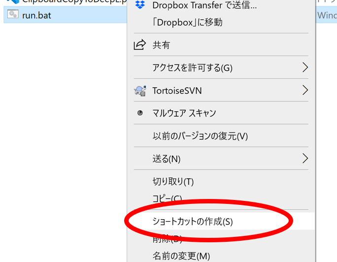
バッチファイルのショートカットを作成します．

ショートカットのプロパティから，ショートカットキーの設定を行います

枠をクリックして割り当てたいキーを打つと勝手に入力されます．

（追記: 自分はこのショートカットをC:\ProgramData\Microsoft\Windows\Start Menu\Programs\以下に配置すると使えるようになりました．）

終わりに

これで論文が読むのが捗りますね．

　 Tweet
Qiitaで続きを読む

投稿日：2020-05-15T21:20:51+09:00

論文の文章をショートカットキー1回で整形してDeepL翻訳に突っ込む

英語論文を読むとき一番大変なことといえば，DeepL翻訳にかけるために文をコピーした後，毎回整形することじゃないですか．(?)
その処理を自動化してショートカットキー一つで出来るようにしました．

こんな感じです．Windowsを対象としています．

方法

Pythonスクリプトでクリップボードに格納されている文を取り出し，整形した後DeepL翻訳に投げます．

このPythonスクリプトをバッチファイルから実行できるようにし，

そのバッチファイルをショートカットキーから実行できるようにします．

Pythonスクリプト
ClipboardCopyToDeepL.py
import pyperclip
import webbrowser

text = pyperclip.paste().replace("\n", " ").replace("- ", "")
webbrowser.open("https://www.deepl.com/en/translator#en/ja/"+text.replace(" ", "%20"))
（追記：間違っていたので，正規表現を使わない形に変更しました．）

いたってシンプルですが，pyperclipを使ってクリップボード上のテキストを取り出した後整形しています．
整形のルールは

英単語が改行で区切られている時に入る-をなくす

改行をスペースに置き換える

だけです．
最後にDeepL翻訳にWebリクエストを投げて終わりです．
DeepL翻訳はhttps://www.deepl.com/en/translator#en/ja/の末尾に翻訳したい文字列を入れてあげると翻訳結果が表示されるサイトに飛んでくれるのでそれを利用しました．

このスクリプトをどこかに保存しておいて，バッチファイルでリクエストがあったときに実行されるようにします．

バッチファイル

pythonスクリプトと同じ階層に以下のバッチファイルを配置します
"Pythonの実行ディレクトリ" "pythonスクリプトのディレクトリ"
例えばanacondaを利用しており，作成したスクリプトをデスクトップの"ClipboardCopyToDeepL/"以下に置いた場合は
ClipboardCopyToDeepL.bat
C:\Users\ユーザ名\anaconda3\python.exe C:\Users\ユーザ名\Desktop\ClipboardCopyToDeepL\ClipboardCopyToDeepL.py
となります．

ショートカットキー割り当て

バッチファイルのショートカットを作成します．

ショートカットのプロパティから，ショートカットキーの設定を行います

枠をクリックして割り当てたいキーを打つと勝手に入力されます．

（追記: 自分はこのショートカットをC:\ProgramData\Microsoft\Windows\Start Menu\Programs\以下に配置すると使えるようになりました．）

終わりに

これで論文が読むのが捗りますね．

　 Tweet
Qiitaで続きを読む

投稿日：2020-05-15T21:04:00+09:00

好きな芸能人のテレビ出演情報をLINEに通知する

目的

好きなアイドル、お笑い芸人がテレビに出演しているのを見逃してしまうので、LINEで通知するようにしました。

概要

Yahoo!テレビ Gガイドからテレビ番組の情報を取得し、LINENotifyを使って通知を行いました。毎朝9時にRaspberrypiでプログラムを実行するように設定しました。

番組情報取得

例えば、「眉村ちあき」の地上波の番組(地域設定東京)の場合はこのようなURLです。
https://tv.yahoo.co.jp/search/?q=眉村ちあき&g=0&a=23&oa=1&s=1

tv_information(query,romaji,jenre)という関数を定義し、入力として通知したい芸能人の名前、出演番組を記録するテキストファイル名、通知したいtv番組のジャンルを受け取ります。入力に応じたURLから情報を取得しました。今回は東京の地上波の番組に限定しています。
お笑いコンビ、ニューヨークの情報を通知したかったのですがニューヨークのワードではアメリカの州のニューヨークに関連した番組がたくさん通知されてしまうので、番組のジャンルを指定して通知できるようにしています。すべてのジャンルはjenre=0、バラエティーはgenre=5を入力します。

LINE

LINE Notify
ここからトークンを取得しました。
line_notify_token = "取得したLINE API"のところに取得したトークンを入力します。

使ったコード

tv_line.py

import requests
from bs4 import BeautifulSoup
import sys
from time import sleep

#テレビの情報を取得する(引数: 出演者の名前、ローマ字(ファイル名にする)、ジャンル)
def tv_information(query,romaji,jenre):
#すべてのジャンルなら0、バラエティーに絞るなら5
    if jenre==0:
        no=''
    elif jenre==5:
        no='05'
    url = "https://tv.yahoo.co.jp/search/?q="+query+"&g="+no+"&a=23&oa=1&s=1" 
    res = requests.get(url)
    status = res.status_code

    #Requestsのステータスコードが200でなければLINEに通知して終了する
    if status != 200:
        def LineNotify(message):
            line_notify_token = "取得したLINE API"
            line_notify_api = "https://notify-api.line.me/api/notify"
            payload = {"message": message}
            headers = {"Authorization": "Bearer " + line_notify_token}
            requests.post(line_notify_api, data=payload, headers=headers)
        message = "Requestsに失敗しました"
        LineNotify(message)
        sys.exit()


    #ステータスコードが200ならば処理継続
    else:
        pass

    #キーワード検索数を取得
    soup = BeautifulSoup(res.text,"html.parser")
    p = soup.find("p",class_="floatl pt5p")

    #検索数が0ならば処理終了
    if p == None:
        print('0')
        non={}
        return non  

    #検索数が1以上ならば処理継続
    else:
        pass

    answer = int(p.em.text) #検索数
    page = 1
    list1 = []  #放送日時
    list2 = []  #放送局
    list3 = []  #番組タイトル

    #ページごとに情報取得
    while answer > 0:
        url = "https://tv.yahoo.co.jp/search/?q="+query+"&g="+no+"&a=23&oa=1&s="+str(page)
        res = requests.get(url)
        soup = BeautifulSoup(res.text, "html.parser")

        dates = soup.find_all("div",class_="leftarea")
        for date in dates:
            d = date.text
            d = ''.join(d.splitlines())
            list1.append(d)

        for s in soup("span",class_="floatl"):
            s.decompose()
        tvs = soup.find_all("span",class_="pr35")
        for tv in tvs:
            list2.append(tv.text)

        titles = soup.find_all("div",class_="rightarea")
        for title in titles:
            t = title.a.text
            list3.append(t)

        page = page + 10
        answer = answer - 10

        sleep(3)

    #list1～list3から放送日時＋放送局＋番組タイトルをまとめたlist_newの作成
    list_new = [x +" "+ y for (x , y) in zip(list1,list2)]
    list_new = [x +" "+ y for (x , y) in zip(list_new,list3)]
    filename=romaji+'.txt'
    #テキストファイルから前回のデータを集合として展開する
    f = open(filename,'r') 
    f_old = f.read()
    list_old = f_old.splitlines()   
    set_old = set(list_old)         
    f.close()           

    f = open(filename, 'w') 
    for x in list_new:
        f.write(str(x)+"\n")    #ファイル書き込み
    f.close()   

    #前回のデータと今回のデータの差集合をとる
    set_new = set(list_new)
    set_dif = set_new - set_old
    return set_dif

def LINE_notify(set_dif,query,romaji):

    #差集合がなければ処理終了
    if len(set_dif) == 0:
        return  

    #差集合があればリストとして取り出してLINEに通知する
    else:
        list_now = list(set_dif)
        list_now.sort()

        for L in list_now:
            def LineNotify(message):
                line_notify_token = "取得したLINE API"
                line_notify_api = "https://notify-api.line.me/api/notify"
                payload = {"message": message}
                headers = {"Authorization": "Bearer " + line_notify_token}
                requests.post(line_notify_api, data=payload, headers=headers)
            message = query+"の出演番組情報\n\n" + L
            LineNotify(message)
            sleep(2)
        return

# すべてのジャンルの眉村ちあきの出演番組を通知
set_dif1=tv_information('眉村ちあき','mayumura',0)
LINE_notify(set_dif1,'眉村ちあき','mayumura')

# すべてのジャンルの空気階段の出演番組を通知
set_dif2=tv_information('空気階段','kuuki',0)
LINE_notify(set_dif2,'空気階段','kuuki')

# バラエティーのジャンルのニューヨークの出演番組を通知
set_dif3=tv_information('ニューヨーク','newy',5)
LINE_notify(set_dif3,'ニューヨーク','newy')

実行

毎日朝9時にRaspberrypiでこのプログラムを実行するようにしました。
crontab -eでファイルに以下の文を書き込みました。

00 09 * * * python3 /home/pi/tv_line.py

実行時間の後にジョブを書きます。実行時間は、分、時、日、月、曜日の順で書きます。

参考

Yahooテレビ番組表から情報取得(Webスクレイピング初級)
浜辺美波の出演番組をスクレイピングで取得
 crontabコマンドについてまとめました【Linuxコマンド集】

　 Tweet
Qiitaで続きを読む

投稿日：2020-05-15T20:58:16+09:00

Pythonを使ってCovid-19(コロナ)のデータを分析しよう【初心者向け】

海外youtubeで、Pythonを使って、Covid-19(コロナ)の感染者数などのデータを使ってデータ分析をするレクチャー動画があったのでやってみました。

出典動画はこちら↓
Analyzing Coronavirus with Python (COVID-19) by NeuralNine on Youtube

対象

Pythonの初心者で、Pandasに慣れたいデータ分析をしてみたい方に特におすすめです。
レクチャーは英語ですが、とても平易かつ丁寧な解説なので是非見てみて下さい。

本記事について

Jupyter notebook上で日本語でコメントを入れながら、当該動画の演習を行いました。実際に動画を見ながら演習を行うのがおすすめですが、英語が苦手な方やデータ分析の流れを把握したい方が、ざっとこの記事を読むだけでもイメージをつかめるように書いています。

リアルデータ(※出典は後述)を利用していますが、データ分析プロセスとしては特にシャープな分析結果を目的としているものではなく、(Pandasライブラリ等の)演習に重きを置いたものになります。

2020/5/1までのデータを利用しています。(※レクチャー動画は、撮影時の3/22までのデータ)

演習

 Analyzing Coronavirus with Python (COVID-19) by NeuralNine on Youtube

データセットは以下のサイトからダウンロード

HDX(HUMANITARIAN DATA EXCHANGE)

リンク先のデータセットの以下のものを使用

- time_series_covid19_confirmed_global.csv
- time_series_covid19_deaths_global.csv
- time_series_covid19_recovered_global.csv

【感染(確認)者,死者数,回復者数】のデータです。

データの名前が長いので、以下のように変更します。
- time_series_covid19_confirmed_global.csv → covid_confirmed.csv
- time_series_covid19_deaths_global.csv → covid_deaths.csv
- time_series_covid19_recovered_global.csv → covid_recovered.csv

ライブラリをインポート
import pandas as pd
import matplotlib.pyplot as plt

%matplotlib inline
データを読み込みます
confirmed = pd.read_csv("covid19_confirmed.csv")
deaths = pd.read_csv("covid19_deaths.csv")
recovered = pd.read_csv("covid19_recovered.csv")
試しに感染者のデータを表示させます(※ 元の動画では、撮影時時点の3/22のデータですが、以下は5/1まで)
confirmed.head()
Province/State Country/Region Lat Long 1/22/20 1/23/20 1/24/20 1/25/20 1/26/20 1/27/20 ... 4/22/20 4/23/20 4/24/20 4/25/20 4/26/20 4/27/20 4/28/20 4/29/20 4/30/20 5/1/20

0 NaN Afghanistan 33.0000 65.0000 0 0 0 0 0 0 ... 1176 1279 1351 1463 1531 1703 1828 1939 2171 2335

1 NaN Albania 41.1533 20.1683 0 0 0 0 0 0 ... 634 663 678 712 726 736 750 766 773 782

2 NaN Algeria 28.0339 1.6596 0 0 0 0 0 0 ... 2910 3007 3127 3256 3382 3517 3649 3848 4006 4154

3 NaN Andorra 42.5063 1.5218 0 0 0 0 0 0 ... 723 723 731 738 738 743 743 743 745 745

4 NaN Angola -11.2027 17.8739 0 0 0 0 0 0 ... 25 25 25 25 26 27 27 27 27 30

5 rows × 105 columns

※ 緯度(Lat),経度(Long)

今回は、ProvinceとLat/Longはあまり必要でないので、列ごと消します
confirmed = confirmed.drop(['Province/State','Lat','Long'],axis=1)
deaths = deaths.drop(['Province/State','Lat','Long'],axis=1)
recovered = recovered.drop(['Province/State','Lat','Long'],axis=1)
このデータを、Country/Regionごとに集計してみましょう
confirmed = confirmed.groupby(confirmed["Country/Region"]).aggregate("sum")
deaths = deaths.groupby(deaths["Country/Region"]).aggregate("sum")
recovered = recovered.groupby(recovered["Country/Region"]).aggregate("sum")
confirmed.head()
1/22/20 1/23/20 1/24/20 1/25/20 1/26/20 1/27/20 1/28/20 1/29/20 1/30/20 1/31/20 ... 4/22/20 4/23/20 4/24/20 4/25/20 4/26/20 4/27/20 4/28/20 4/29/20 4/30/20 5/1/20

Country/Region

Afghanistan 0 0 0 0 0 0 0 0 0 0 ... 1176 1279 1351 1463 1531 1703 1828 1939 2171 2335

Albania 0 0 0 0 0 0 0 0 0 0 ... 634 663 678 712 726 736 750 766 773 782

Algeria 0 0 0 0 0 0 0 0 0 0 ... 2910 3007 3127 3256 3382 3517 3649 3848 4006 4154

Andorra 0 0 0 0 0 0 0 0 0 0 ... 723 723 731 738 738 743 743 743 745 745

Angola 0 0 0 0 0 0 0 0 0 0 ... 25 25 25 25 26 27 27 27 27 30

5 rows × 101 columns

そして、次に、日付が特徴量となっていますが、今回は国を特徴量にしたいため、データを転置(行列入れ替え)します。
confirmed = confirmed.T
deaths = deaths.T
recovered = recovered.T
confirmed.head()
Country/Region Afghanistan Albania Algeria Andorra Angola Antigua and Barbuda Argentina Armenia Australia Austria ... United Kingdom Uruguay Uzbekistan Venezuela Vietnam West Bank and Gaza Western Sahara Yemen Zambia Zimbabwe

1/22/20 0 0 0 0 0 0 0 0 0 0 ... 0 0 0 0 0 0 0 0 0 0

1/23/20 0 0 0 0 0 0 0 0 0 0 ... 0 0 0 0 2 0 0 0 0 0

1/24/20 0 0 0 0 0 0 0 0 0 0 ... 0 0 0 0 2 0 0 0 0 0

1/25/20 0 0 0 0 0 0 0 0 0 0 ... 0 0 0 0 2 0 0 0 0 0

1/26/20 0 0 0 0 0 0 0 0 4 0 ... 0 0 0 0 2 0 0 0 0 0

5 rows × 187 columns

ここまでで、データの下準備は一旦整いました。計算に移っていきます。

まず、感染者数の増加数の推移をみていきましょう

ここで必要になってくるデータは当該日とその前日の感染者数の差です。
new_cases = confirmed.copy()
for day in range(1,len(confirmed)):
    new_cases.iloc[day] = confirmed.iloc[day] - confirmed.iloc[day - 1]
直近の10日分のデータを見ます
new_cases.tail(10)
Country/Region Afghanistan Albania Algeria Andorra Angola Antigua and Barbuda Argentina Armenia Australia Austria ... United Kingdom Uruguay Uzbekistan Venezuela Vietnam West Bank and Gaza Western Sahara Yemen Zambia Zimbabwe

4/22/20 84 25 99 6 1 1 113 72 7 52 ... 4466 8 38 3 0 8 0 0 4 0

4/23/20 103 29 97 0 0 0 291 50 10 77 ... 4608 14 42 23 0 6 0 0 2 0

4/24/20 72 15 120 8 0 0 172 73 15 69 ... 5394 6 46 7 2 4 0 0 8 1

4/25/20 112 34 129 7 0 0 173 81 17 77 ... 4929 33 58 5 0 -142 0 0 0 2

4/26/20 68 14 126 0 1 0 112 69 20 77 ... 4468 10 7 2 0 0 0 0 4 0

4/27/20 172 10 135 5 1 0 111 62 7 49 ... 4311 14 35 4 0 0 0 0 0 1

4/28/20 125 14 132 0 0 0 124 59 23 83 ... 4002 5 35 0 0 1 0 0 7 0

4/29/20 111 16 199 0 0 0 158 65 8 45 ... 4091 5 63 2 0 1 0 5 2 0

4/30/20 232 7 158 2 0 0 143 134 14 50 ... 6040 13 37 2 0 0 0 0 9 8

5/1/20 164 9 148 0 3 1 104 82 12 79 ... 6204 5 47 2 0 9 0 1 3 0

10 rows × 187 columns

感染者データと比べてみましょう
confirmed.tail(10)
Country/Region Afghanistan Albania Algeria Andorra Angola Antigua and Barbuda Argentina Armenia Australia Austria ... United Kingdom Uruguay Uzbekistan Venezuela Vietnam West Bank and Gaza Western Sahara Yemen Zambia Zimbabwe

4/22/20 1176 634 2910 723 25 24 3144 1473 6652 14925 ... 134638 543 1716 288 268 474 6 1 74 28

4/23/20 1279 663 3007 723 25 24 3435 1523 6662 15002 ... 139246 557 1758 311 268 480 6 1 76 28

4/24/20 1351 678 3127 731 25 24 3607 1596 6677 15071 ... 144640 563 1804 318 270 484 6 1 84 29

4/25/20 1463 712 3256 738 25 24 3780 1677 6694 15148 ... 149569 596 1862 323 270 342 6 1 84 31

4/26/20 1531 726 3382 738 26 24 3892 1746 6714 15225 ... 154037 606 1869 325 270 342 6 1 88 31

4/27/20 1703 736 3517 743 27 24 4003 1808 6721 15274 ... 158348 620 1904 329 270 342 6 1 88 32

4/28/20 1828 750 3649 743 27 24 4127 1867 6744 15357 ... 162350 625 1939 329 270 343 6 1 95 32

4/29/20 1939 766 3848 743 27 24 4285 1932 6752 15402 ... 166441 630 2002 331 270 344 6 6 97 32

4/30/20 2171 773 4006 745 27 24 4428 2066 6766 15452 ... 172481 643 2039 333 270 344 6 6 106 40

5/1/20 2335 782 4154 745 30 25 4532 2148 6778 15531 ... 178685 648 2086 335 270 353 6 7 109 40

10 rows × 187 columns

例えば、AfghanistanやAlgeriaやArgentinaやUnited Kingdomは、感染者数の絶対数も多いですが、新規感染者数も依然多いということが分かります。

new_casesでは、感染者数の日別の"増加数"を見ましたが、次に"増加率"を見ましょう。

(当該日の増加数 / 前日の感染者数) * 100 で増加率を出すことが出来ます
growth_rate = confirmed.copy()

for day in range(1,len(growth_rate)):
    growth_rate.iloc[day] = ( new_cases.iloc[day] / confirmed.iloc[day-1] ) * 100
growth_rate.tail(10)
Country/Region Afghanistan Albania Algeria Andorra Angola Antigua and Barbuda Argentina Armenia Australia Austria ... United Kingdom Uruguay Uzbekistan Venezuela Vietnam West Bank and Gaza Western Sahara Yemen Zambia Zimbabwe

4/22/20 7.692308 4.105090 3.521878 0.836820 4.166667 4.347826 3.728143 5.139186 0.105342 0.349627 ... 3.430845 1.495327 2.264601 1.052632 0.000000 1.716738 0.0 0.000000 5.714286 0.000000

4/23/20 8.758503 4.574132 3.333333 0.000000 0.000000 0.000000 9.255725 3.394433 0.150331 0.515913 ... 3.422511 2.578269 2.447552 7.986111 0.000000 1.265823 0.0 0.000000 2.702703 0.000000

4/24/20 5.629398 2.262443 3.990688 1.106501 0.000000 0.000000 5.007278 4.793171 0.225158 0.459939 ... 3.873720 1.077199 2.616610 2.250804 0.746269 0.833333 0.0 0.000000 10.526316 3.571429

4/25/20 8.290155 5.014749 4.125360 0.957592 0.000000 0.000000 4.796230 5.075188 0.254605 0.510915 ... 3.407771 5.861456 3.215078 1.572327 0.000000 -29.338843 0.0 0.000000 0.000000 6.896552

4/26/20 4.647984 1.966292 3.869779 0.000000 4.000000 0.000000 2.962963 4.114490 0.298775 0.508318 ... 2.987250 1.677852 0.375940 0.619195 0.000000 0.000000 0.0 0.000000 4.761905 0.000000

4/27/20 11.234487 1.377410 3.991721 0.677507 3.846154 0.000000 2.852004 3.550974 0.104260 0.321839 ... 2.798678 2.310231 1.872659 1.230769 0.000000 0.000000 0.0 0.000000 0.000000 3.225806

4/28/20 7.339988 1.902174 3.753199 0.000000 0.000000 0.000000 3.097677 3.263274 0.342211 0.543407 ... 2.527345 0.806452 1.838235 0.000000 0.000000 0.292398 0.0 0.000000 7.954545 0.000000

4/29/20 6.072210 2.133333 5.453549 0.000000 0.000000 0.000000 3.828447 3.481521 0.118624 0.293026 ... 2.519864 0.800000 3.249097 0.607903 0.000000 0.291545 0.0 500.000000 2.105263 0.000000

4/30/20 11.964930 0.913838 4.106029 0.269179 0.000000 0.000000 3.337223 6.935818 0.207346 0.324633 ... 3.628914 2.063492 1.848152 0.604230 0.000000 0.000000 0.0 0.000000 9.278351 25.000000

5/1/20 7.554123 1.164295 3.694458 0.000000 11.111111 4.166667 2.348690 3.969022 0.177357 0.511261 ... 3.596918 0.777605 2.305051 0.600601 0.000000 2.616279 0.0 16.666667 2.830189 0.000000

10 rows × 187 columns

さて、感染者数(confirmed)はいわゆる累計の数なので、一旦ここで、現在進行形の感染者数(Active)を出しましょう。

【感染者数(confirmed)】から【死者数(deaths)と回復者数(recovered)】を引くと、【現在進行形の感染者数(Active)】が計算できそうです。
active_cases = confirmed.copy()

for day in range(0,len(confirmed)):
    active_cases.iloc[day] = confirmed.iloc[day] - deaths.iloc[day] - recovered.iloc[day]
そして、この現在進行形の感染者数active_casesのデータを利用して、再度、現在進行形の感染者数の増加率を調べましょう。

これを調べることによって、収束していそうかどうかが分かりそうです。
overall_growth_rate = confirmed.copy()

for day in range(0,len(confirmed)):
    overall_growth_rate.iloc[day] = ((active_cases.iloc[day] - active_cases.iloc[day-1]) / active_cases.iloc[day-1]) * 100
overall_growth_rate.tail(10)
Country/Region Afghanistan Albania Algeria Andorra Angola Antigua and Barbuda Argentina Armenia Australia Austria ... United Kingdom Uruguay Uzbekistan Venezuela Vietnam West Bank and Gaza Western Sahara Yemen Zambia Zimbabwe

4/22/20 7.064018 5.462185 2.920284 -5.276382 6.250000 -15.384615 3.718200 6.250000 -12.214551 -9.498681 ... 3.270797 -1.895735 -4.258555 -1.265823 -13.461538 2.046036 0.000000 0.000000 12.500000 -4.347826

4/23/20 9.072165 0.000000 -4.524540 -6.366048 0.000000 0.000000 10.896226 2.941176 -6.836056 -9.750567 ... 3.411790 -7.729469 -5.480540 12.179487 -2.222222 -3.759398 -83.333333 0.000000 0.000000 0.000000

4/24/20 5.860113 2.390438 4.738956 -1.699717 0.000000 -9.090909 4.423650 0.119048 -5.064935 -4.199569 ... 3.743980 -4.712042 -1.260504 0.571429 13.636364 1.041667 0.000000 -100.000000 22.222222 4.545455

4/25/20 9.642857 9.727626 4.141104 2.017291 0.000000 0.000000 4.480652 0.594530 -15.321477 -5.994755 ... 3.332975 16.483516 -2.382979 2.840909 -10.000000 -36.082474 0.000000 NaN 0.000000 8.695652

4/26/20 3.745928 2.127660 6.701031 0.000000 5.882353 0.000000 1.091618 4.609929 -11.954766 -4.304504 ... 3.232666 1.886792 -6.538797 -1.657459 0.000000 3.629032 0.000000 NaN -2.272727 0.000000

4/27/20 11.930926 -0.694444 5.383023 -10.169492 5.555556 0.000000 2.815272 5.197740 -3.669725 -1.582674 ... 3.051680 1.388889 -6.343284 -0.561798 0.000000 0.000000 0.000000 NaN 0.000000 -8.000000

4/28/20 8.134642 1.048951 2.226588 -4.402516 0.000000 0.000000 3.450863 4.296455 -5.714286 -6.559458 ... 2.318102 -1.369863 -6.474104 0.000000 6.666667 5.058366 0.000000 NaN 16.279070 0.000000

4/29/20 5.512322 -2.768166 9.032671 -8.552632 -5.263158 0.000000 4.387237 3.192585 -4.444444 -7.472826 ... 2.386758 -6.018519 -4.472843 1.129944 0.000000 0.370370 0.000000 inf -20.000000 0.000000

4/30/20 13.521819 -3.202847 4.406580 -15.467626 0.000000 0.000000 2.605071 10.279441 -1.585624 -4.013705 ... 3.845988 2.955665 0.000000 -2.234637 6.250000 -1.845018 0.000000 -40.000000 20.000000 34.782609

5/1/20 5.955604 -3.308824 5.796286 -0.425532 -5.555556 -30.000000 2.064997 2.986425 -2.255639 -6.578276 ... 3.750518 -6.220096 -3.567447 1.142857 0.000000 3.383459 0.000000 33.333333 -33.333333 0.000000

10 rows × 187 columns

直近10日(2020/04/22-05/01)の現在進行形の感染者数の増加率 (中国・イタリア・アメリカ・日本)

※ ちょこっと、ここの部分にオリジナルの加えています。

まず、コロナ発症国と考えられている中国は、最近収束しているみたいなので、中国の直近10日のデータを見てみましょう
overall_growth_rate['China'].tail(10)
4/22/20   -3.314528
4/23/20   -7.731583
4/24/20   -8.774704
4/25/20   -4.852686
4/26/20   -9.107468
4/27/20   -9.118236
4/28/20   -2.866593
4/29/20   -5.448354
4/30/20   -4.441777
5/1/20    -5.904523
Name: China, dtype: float64
増加率マイナス、つまり現在進行形の感染者数が減り続けている　→　収束に向かっていることが分かります。

次に、イタリアはどうでしょうか。
overall_growth_rate['Italy'].tail(10)
4/22/20   -0.009284
4/23/20   -0.790165
4/24/20   -0.300427
4/25/20   -0.638336
4/26/20    0.241859
4/27/20   -0.273319
4/28/20   -0.574599
4/29/20   -0.520888
4/30/20   -2.967790
5/1/20    -0.598714
Name: Italy, dtype: float64
1%未満の減少率なので微減ですが、増えてはいません。
overall_growth_rate['US'].tail(10)
4/22/20    3.470050
4/23/20    3.307839
4/24/20    2.102556
4/25/20    3.874078
4/26/20    2.536775
4/27/20    2.064644
4/28/20    2.166569
4/29/20    2.377575
4/30/20   -0.668941
5/1/20     2.583283
Name: US, dtype: float64
アメリカは、まだ数%ずつ増加しています。
overall_growth_rate['Japan'].tail(10)
4/22/20    2.512198
4/23/20    6.794937
4/24/20    3.868765
4/25/20    2.382691
4/26/20    0.401248
4/27/20    5.408526
4/28/20   -3.589182
4/29/20   -2.875120
4/30/20    0.755803
5/1/20    -2.884444
Name: Japan, dtype: float64
日本も、ちょっとずつ直近で減ってきた感じはありますが、増加傾向にあります。

日本は、せっかくなので、直近10日の増加率の平均を見てみましょう。
overall_growth_rate['Japan'].tail(10).mean()
1.277542288600591
1%程度ですが、増加傾向にある感じです。まぁ、日本はまだ感染者数も少ないので、比較的抑えられているといえるかもしれません。

ここから可視化(visualization)を交えていきます。

最初に死亡率を見ていきましょう。死亡率は、地域ごとのコロナの深刻さを表す指標となるので重要です。

まず、死亡率のデータフレームは、先ほどの手順とほぼ同様です。死亡率は、死亡者/感染者で表されます。
death_rate = confirmed.copy()
for day in range(0,len(confirmed)):
    death_rate.iloc[day] = (deaths.iloc[day] / confirmed.iloc[day]) * 100
次に、必要な必要なベッド台数(逆に、どれだけ不足が生じそうか)を算出します。

感染者のうち病院が必要な人の割合である入院率"hospitalization"を用います。これは、正しい数値は、分からないので、一旦仮の数値(ここでは、0.05)を用います。好きな数字に変えても大丈夫です。このレクチャーでは、分析・計算手法にフォーカスするため、一旦正確さは置いておきます。

※ちなみに、入院率は、コロナ陽性かつ入院が必要な人のことで、残りの95%は陽性であっても、入院(ベッド)は必要ではないとみなしています。
hospitalization_rate_estimate = 0.05
hospitalization_needed = confirmed.copy()
for day in range(0,len(confirmed)):
    hospitalization_needed.iloc[day] = active_cases.iloc[day] * hospitalization_rate_estimate
hospitalization_needed.tail()
Country/Region Afghanistan Albania Algeria Andorra Angola Antigua and Barbuda Argentina Armenia Australia Austria ... United Kingdom Uruguay Uzbekistan Venezuela Vietnam West Bank and Gaza Western Sahara Yemen Zambia Zimbabwe

4/27/20 71.30 14.30 76.35 15.90 0.95 0.50 133.30 46.55 52.50 118.15 ... 6654.15 10.95 50.20 8.85 2.25 12.85 0.05 0.00 2.15 1.15

4/28/20 77.10 14.45 78.05 15.20 0.95 0.50 137.90 48.55 49.50 110.40 ... 6808.40 10.80 46.95 8.85 2.40 13.50 0.05 0.00 2.50 1.15

4/29/20 81.35 14.05 85.10 13.90 0.90 0.50 143.95 50.10 47.30 102.15 ... 6970.90 10.15 44.85 8.95 2.40 13.55 0.05 0.25 2.00 1.15

4/30/20 92.35 13.60 88.85 11.75 0.90 0.50 147.70 55.25 46.55 98.05 ... 7239.00 10.45 44.85 8.75 2.55 13.30 0.05 0.15 2.40 1.55

5/1/20 97.85 13.15 94.00 11.70 0.85 0.35 150.75 56.90 45.50 91.60 ... 7510.50 9.80 43.25 8.85 2.55 13.75 0.05 0.20 1.60 1.55

5 rows × 187 columns

一旦、ここで国をひとつ取り出しても、どれだけ深刻かわかりづらいため、一旦直近5日の平均を見ます。
hospitalization_needed.tail().mean().mean()
532.5691978609626
直近５日のすべての国の必要ベッド数の平均です。ばらつきも当然あるため、あまり理想的な参考値ではないですが、一旦これを参考とします。

イタリアの直近5日の平均を見てみましょう。
hospitalization_needed['Italy'].tail().mean()
5181.6900000000005
つまり、ざっと世界中の平均の10倍という数値が出ました。かなり深刻です。

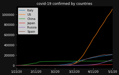
可視化します。ただ、国が多すぎるので、今回は、いくつか任意の国を選びましょう。ここでは、イタリア、アメリカ、中国、日本、ロシアスペインを選びます。
countries = ['Italy','US',"China","Japan","Russia","Spain"]
ax = plt.subplot()
ax.set_facecolor("black")
ax.figure.set_facecolor("#121212")
ax.tick_params(axis="x",colors="white")
ax.tick_params(axis="y",colors="white")
ax.set_title("covid-19 confirmed by countries",color="white")

for country in countries:
    confirmed[country].plot(label=country)
plt.legend(loc="upper left")
plt.show()
USが3月末ぐらいから著しく感染者が増えていますね。

死者数を見ましょう。

グラフの形はあまり変わらず、感染者数に伴っているような感じです。

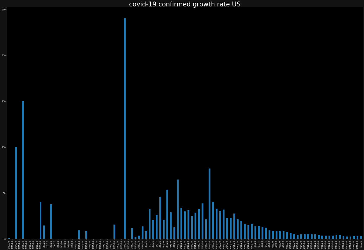
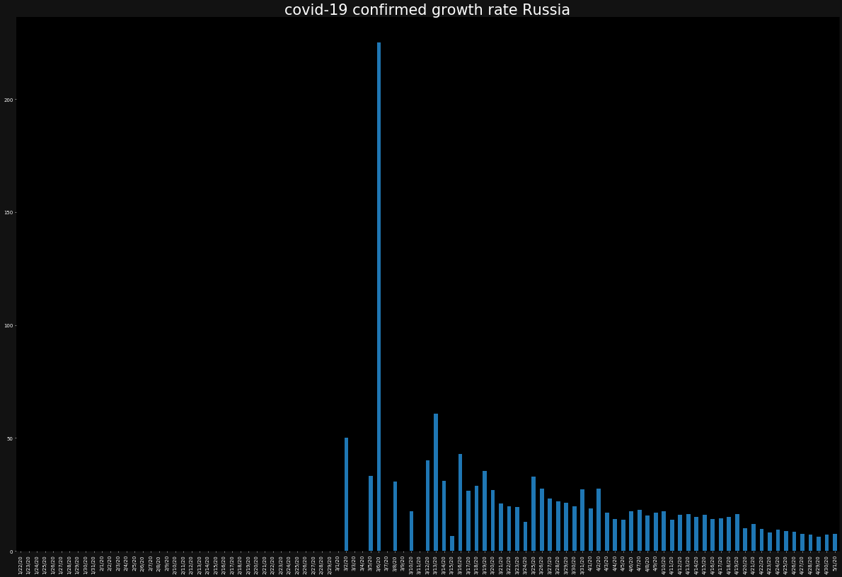
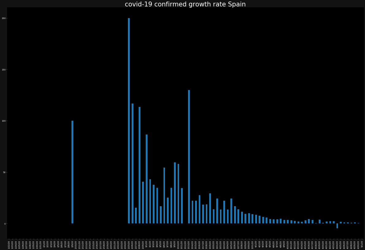
次に、感染者の増加率をプロットしてみましょう。

ただし、今度は、バーチャートでプロットします。また、バーチャートではあまりひとつの図にグラフが重なりすぎると、可視性が低くなるため別々に表示します。
for country in countries:
    ax = plt.subplot()
    ax.set_facecolor("black")
    ax.figure.set_facecolor("#121212")
    ax.tick_params(axis="x",colors="white")
    ax.tick_params(axis="y",colors="white")
    ax.set_title(f"covid-19 confirmed growth rate {country}",color="white")
    growth_rate[country].plot.bar() 
    plt.show()
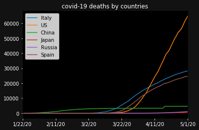
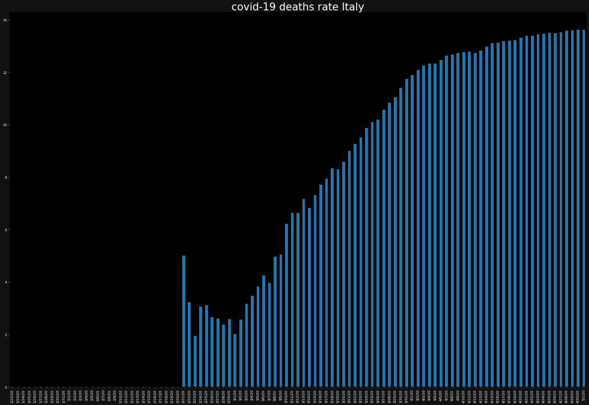
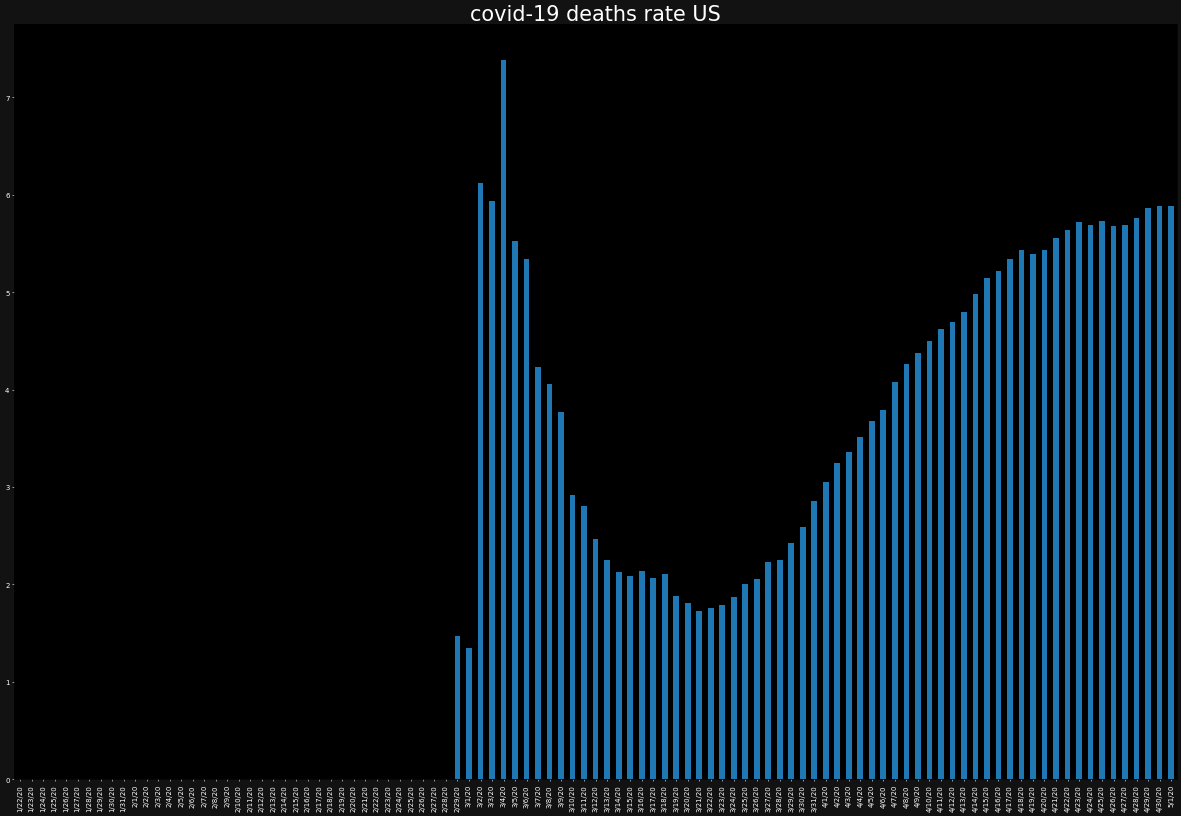
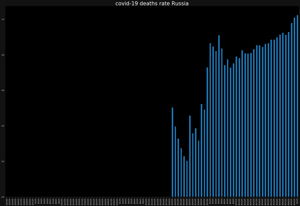
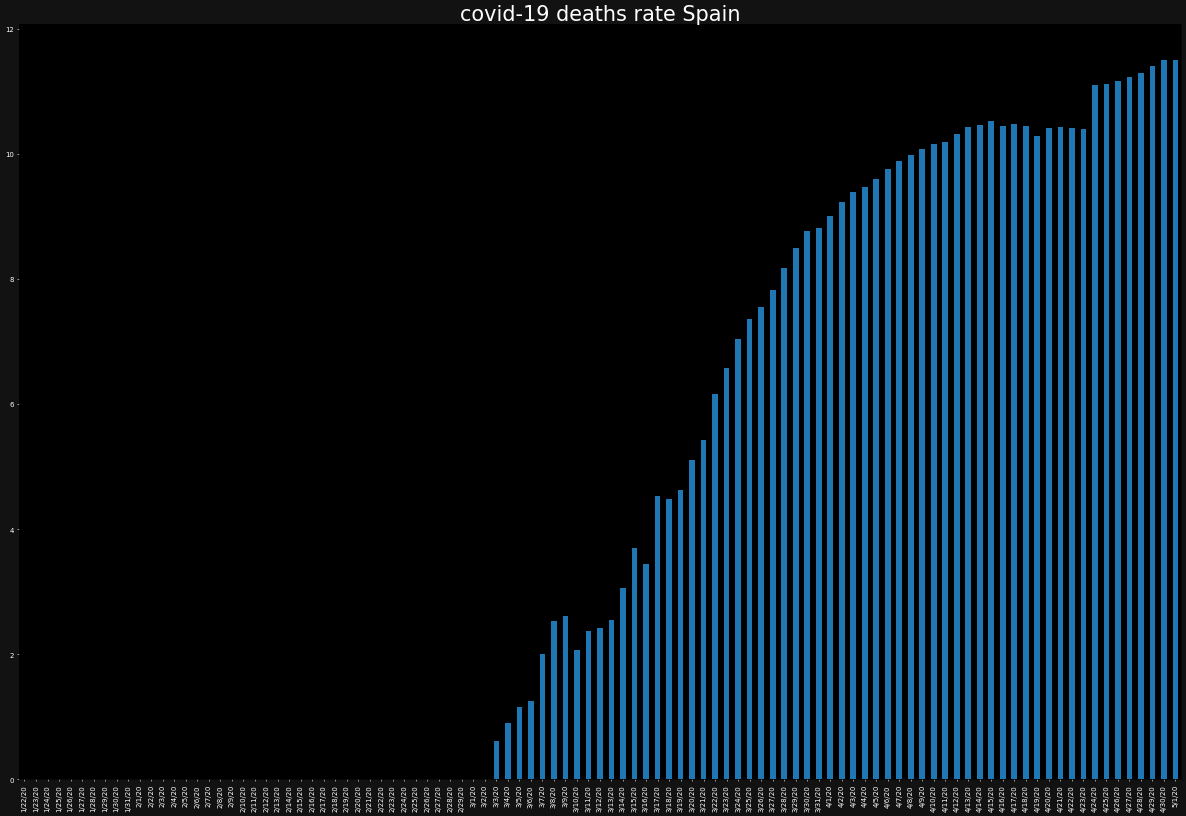
同じ要領で死者数の感染数、死亡率(※上記は、"感染者の増加率"でこちらは"死亡率"です)も見ましょう。
ax = plt.subplot()
ax.set_facecolor("black")
ax.figure.set_facecolor("#121212")
ax.tick_params(axis="x",colors="white")
ax.tick_params(axis="y",colors="white")
ax.set_title("covid-19 deaths by countries",color="white")

for country in countries:
    deaths[country].plot(label=country)
plt.legend(loc="upper left")
plt.show()
for country in countries:
    ax = plt.subplot()
    ax.set_facecolor("black")
    ax.figure.set_facecolor("#121212")
    ax.tick_params(axis="x",colors="white")
    ax.tick_params(axis="y",colors="white")
    ax.set_title(f"covid-19 deaths rate {country}",color="white")
    death_rate[country].plot.bar() 
    plt.show()
死亡率に国別で差があることが分かります。

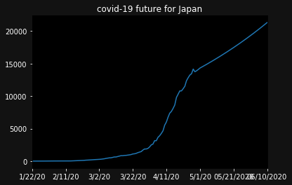
さて、最後に今後のコロナウイルスの影響のシミュレーションに移ります。

一旦、今後、仮値として、日次で1%の感染者が増えるとしましょう。
simulated_growth_rate = 0.01
ここで、予測用のこれからの新しい日付データを追加します。

範囲を指定して、日付データを生成できるdate_rangeメソッドを利用します。

今回用いているデータは、05/01/20が最後なので、その次の日から40日間。
dates = pd.date_range(start="05/02/2020",periods=40,freq='D')
dates = pd.Series(dates)
dates = dates.dt.strftime("%m/%d/%Y")
simulated = confirmed.copy()
simulated = simulated.append(pd.DataFrame(index=dates))

for day in range(len(confirmed),len(confirmed)+40):
    simulated.iloc[day] = simulated.iloc[day-1] * (1 + simulated_growth_rate)
ax = plt.subplot()
ax.set_facecolor("black")
ax.figure.set_facecolor("#121212")
ax.tick_params(axis="x",colors="white")
ax.tick_params(axis="y",colors="white")
ax.set_title(f"covid-19 future for Japan",color="white")
simulated['Japan'].plot()
plt.show()
※ 念押しですが、これは仮の成長率(※ 日次1%ずつ増え続ける)に基づいた数字です。厳密なシミュレーションとして、受け止める必要はありません。

以上です。ちょくちょく引用元の動画と違う部分はありますが、ざっとデータ分析の流れをつかめたかと思います。
是非、元動画をご覧ください。

投稿者のNeuralNine氏は、動画の最後に、この分析は仮の数値などはあるものだから、真剣に受け止めなくていいことは強調したうえで、事実をデータをもとに把握し、自分が意識すべきことは大事であることを伝えてくれていました。

　 Tweet
Qiitaで続きを読む

投稿日：2020-05-15T20:43:39+09:00

【強化学習】R2D2を実装/解説してみたリベンジハイパーパラメータ解説編（Keras-RL）

ハイパーパラメータ解説編です。
各パラメータに関してまとめてみました。

中身のアルゴリズムについてはこちら
【強化学習】R2D2を実装/解説してみたリベンジ解説編（Keras-RL）

コード全体

本記事の対象コードはgithubにあげています。

github

目次

共通パラメータ解説

Rainbow/R2D2特有のパラメータ解説

学習以外の機能の解説

NNモデルの中間層の可視化

動画化

save/load

学習履歴のログ取得

ハイパーパラメータ設定例

DQN(論文)

Keras-RL Cartpoleのサンプル

Rainbow(論文)

R2D2(論文)

共通パラメータ

Rainbow(DQN)とR2D2で共通のパラメータです。

env 依存関係のパラメータ

概要型例備考

input_shape 入力shape tuple (84,84) env.observation_space.shape

input_type 入力形式を指定 InputType InputType.GRAY_2ch 独自実装

image_model 画像層のモデル形式 ImageModel(独自実装) DQNImageModel()

nb_actions アクション数(出力数) int 4 env.action_space.n

processor Gymのカスタム機能を提供するクラス Processor(Keras-rl) None

input_shape
入力形式を tuple で指定します。
画像なら (width, height) の形式ですね。
Gym の場合は env.observation_space.shape で取得できる形式です。

input_type
上記 input_shape を補う指定です。
独自実装しています。
下記の4つの種類を想定しており、input_shape の内容に合わせて指定してください。
InputType
class InputType(enum.Enum):
    VALUES = 1    # 画像無し
    GRAY_2ch = 3  # (width, height)
    GRAY_3ch = 4  # (width, height, 1)
    COLOR = 5     # (width, height, ch)
image_model
前回の記事で解説した内容です。
ただ現状は２種類しかなく、画像じゃない場合は None、画像の場合は DQNImageModel() を指定してください。

nb_actions
出力形式を int で指定します。
これは agent が選択できるアクション数に相当します。
例えば左と右と止まると3個操作方法がある場合は3アクションになります。
Gym の場合は env.action_space.n で取得できます。(Discrete形式のみ)

processor
Gym で提供されている Env に対してカスタマイズ機能を提供するクラスです。(processor(Keras-rl公式))

NN(ニューラルネットワーク)モデル関係のパラメータ

概要型例備考

batch_size バッチサイズ int 32

optimizer 最適化アルゴリズム Optimizer(Keras) Adam(lr=0.0001) Keras実装

metrics 評価関数 array [] Keras実装

input_sequence 入力フレーム数 int 4

dense_units_num Dense層のユニット数 int 512

enable_dueling_network DuelingNetworkを使うかどうか bool True

dueling_network_type DuelingNetworkで使うアルゴリズム DuelingNetwork DuelingNetwork.AVERAGE

lstm_type LSTMを使用する場合の種類 LstmType(独自実装) LstmType.NONE

lstm_units_num LSTM層のユニット数 int 512

lstm_ful_input_length 1学習あたりの入力学習回数 int 4 STATEFULの場合のみ使用

batch_size
ミニバッチ学習で使用する batch サイズです。(batchについてはこちら(Keras公式))
batchサイズを増やすと学習効率および学習速度が上がるという話があります。
ただ、強化学習は教師あり学習と違い、学習データに制限がないため batch サイズを増やすと学習コストが増える(1回の学習での収束速度は上がるが時間はかかるため、新しい経験を模索する回数が減る)ため、あまり増やしすぎない方がいい気もします。
また、batchサイズは 2^n を指定するといいとかなんとか。

optimizer
NNモデルを compile する際に指定する Keras の Optimizer を指定します。
詳細はオプティマイザ（最適化アルゴリズム）の利用方法(Keras公式)等を参考にしてください。

metrics
Keras の評価関数を指定します。使ったときないのであまり分からない…。
詳細は評価関数の利用方法(Keras公式)等を参考にしてください。

input_sequence(以前はwindow_length)
入力に使う observation の数です。
1 で直近の1frameのみを入力とし、4だと直近から4frameまでを入力として使います。
この値を増やすと入力の表現力が増えますが、学習コストは増えます。

dense_units_num
Dense層のユニット数です。
この値を増やすとNNの表現力が増えますが、学習コストは増えます。

enable_dueling_network
DuelingNetworkを有効にするかどうかです。
DuelingNetworkは状態と行動を分けてNNに学習させることで学習効率をあげようというものです。

dueling_network_type
DuelingNetwork で状態と行動を分ける時に使うアルゴリズムです。
以下の３種類から指定できます。
論文では Average が一番いい結果が出たと書いてありました。
DuelingNetwork
class DuelingNetwork(enum.Enum):
    AVERAGE = 0
    MAX = 1
    NAIVE = 2
lstm_type
LSTMを使う場合の種類を指定します。
LSTMを使用すると時系列に関する情報も学習する事が出来ますが学習コストは増えます。
使わない場合は NONE を指定してください。
STATELESS を指定するとDRQN相当のシンプルなLSTM層をNNモデルに追加します。
STATEFUL を指定するとR2D2相当の複雑な処理をするLSTM層をNNモデルに追加します。
STATEFULはSTATELESSに比べて学習効率は上がりますが、学習コストがかなり増えます。
LstmType
class LstmType(enum.Enum):
    NONE = 0
    STATELESS = 1
    STATEFUL = 2
lstm_ful_input_length
STATEFULの学習における1学習あたりの入力学習回数です。
STATEFULで学習する場合、時系列に沿う形で学習回数を増やす事が出来ます。
その時系列に沿った学習回数の数をここで指定します。(詳細は前回の記事を参照)
数字を増やすと学習効率は(多分)上がりますが、学習コストが増えます。

Experience Replay Memory関連

概要型例備考

memory/remote_memory 使用するメモリ Memory(独自実装) ReplayMemory(10000) 下記参照

経験を貯めるメモリの種類を指定します。
DQN では経験したデータは一度メモリに格納します。
その後、メモリの中からランダムに経験を取り出して学習を行います。
メモリから取り出す方法によっていくつか種類があるのでそれについて説明します。

ReplayMemory

DQN で使われているシンプルなメモリです。(以前の記事)
経験データをランダムに取り出します。
ReplayMemory(
    capacity=10_000
)
capacity
メモリに保存する最大容量です。
多いほうがいいですが、多すぎるとPC側の物理メモリが圧迫されるのでほどほどに。

PERGreedyMemory

優先順位付き経験再生における愚直な実装です。
ランダムではなくTD誤差が最大の経験(もっとも学習への反映率が高い)経験を取り出す方法です。
ただ、これはランダム要素がないのですぐ局所解に入る気がしてうまく学習できません…。(なぜ実装した)
PERGreedyMemory(
    capacity=10_000
)
capacity
メモリに保存する最大容量です。

PERProportionalMemory

優先順位付き経験再生におけるProportional Prioritization(比例優先順位付け)のメモリです。
ランダムではなくTD誤差の確率分布にしたがって経験を取り出す方法です。
(TD誤差が多い経験ほど取り出される確率が高くなる)

ReplayMemory(ランダム選択)よりはかなり学習効率が良くなる感じです。
PERGreedyMemory(
    capacity=100000,
    alpha=0.9,
    beta_initial,
    beta_steps,
    enable_is,
)
パラメータは後述します。

PERRankBaseMemory

優先順位付き経験再生におけるRankBase(順位優先付け)のメモリです。
ランダムではなくTD誤差の順位に比例して経験を取り出します。
例えば３つ経験がある場合、1位は50%、2位は33%、3位は17%で選択されるといった感じです。

ReplayMemory(ランダム選択)よりはかなり学習効率が良くなる感じですが、
Proportional との違いはあまり分かりません。
速度的にはこちらの方が少しだけはやくなっているはず…。
PERRankBaseMemory(
    capacity=100000,
    alpha=0.9,
    beta_initial,
    beta_steps, 
    enable_is,
)
パラメータは後述します。

PERProportionalMemoryとPERRankBaseMemoryのパラメータ

概要型例備考

capacity メモリに保存する最大容量 int 1_000_000

alpha 確率反映率 float 0.9 0.0～1.0

beta_initial IS反映率の初期値 float 0.0 0.0～1.0

beta_steps ISの反映率を1.0にするまでのstep数 int 100_000 学習回数に依存

enable_is ISを有効にするか bool True

capacity
メモリに保存する最大容量です。

alpha
Priority/RankBase の反映率です。(0.0～1.0)
0.0で完全ランダム(ReplayMemoryと同様)で、1.0なら確率分布に完全に従います。

ここで重要度サンプリング(IS)の説明をします。
確率分布に従って経験を出す場合、各経験が選ばれる回数に偏りが生じます。
経験の選択回数が偏ると学習にバイアスがかかってしまうので、それを回避するのが重要度サンプリングです。

具体的には、高い確率で選ばれる経験はQ値の更新への反映率を低くし、低い確率で選ばれる経験はQ値の更新への反映率を高くするというものです。

ISを導入することで学習が安定するらしいです。
また、ISはアニーリング(徐々に反映していく)します。

beta_initial
ISの反映率の初期値です。(0.0 でISを使用しない状態、1.0でISを反映した状態)

beta_steps
ISの反映率を1.0にするまでのstep数です。
学習回数を元に指定してください。

enable_is
ISを有効にするかどうかです。

学習関係のパラメータ

概要型例備考

memory_warmup_size/ remote_memory_warmup_size メモリに経験が貯まるまで学習しないサイズ int 1000

target_model_update Targetモデルへの更新間隔 int 10000

gamma Q学習の割引率 float 0.99 0.0～1.0

enable_double_dqn DoubleDQNを使用するか bool True

enable_rescaling rescaling関数を使用するか bool True

rescaling_epsilon rescaling関数で使う定数 float 0.001

priority_exponent 経験の優先度を計算する際の比率 float 0.9 LESTFULのみ使用

burnin_length burn-inの期間 int 2 LESTFULのみ使用

reward_multisteps MultiStep Reward のstep数 int 3

memory_warmup_size / remote_memory_warmup_size
初期状態ではメモリに経験がなく、学習ができません。
ですのでメモリに経験が貯まるまで学習しない期間を作ります。
その期間をここで指定します。
batch_size 以上の値であまり少なすぎない値がいいと思います。
(あまり減らすと初期で偏った経験データがあった場合に局所解に陥る可能性があります)

target_model_update
DQNにおけるTargetNetworkの更新間隔です。
DQNではTargetNetworkという更新専用のQネットワークを用いて更新します。
TargetNetworkは学習は行わず、一定間隔で今のQネットワークをコピーします。
こうすることで更新に使用するQネットワークに時差が生まれて更新が良くなるとのことです。

gamma
Q学習の割引率です。
報酬をどれだけ伝搬させるかを指定します。
まあ、ほぼ1.0に近い値でいいと思います。

enable_double_dqn
DoubleDQNは学習時に最大のQ値を選んで学習していましたが、ノイズ等の影響で過大評価されている可能性があり良くないということで提案された手法です。
DoubleDQNを使うと学習効率が上がる気がします。

enable_rescaling
報酬に対してrescaling関数を使用するか指定します。
rescaling関数を使用すると報酬がある程度丸められるので報酬による学習のブレが抑えられます。

rescaling_epsilon
rescaling関数で使う定数です。
0になるのを防ぐ定数のようでほぼ0に近い値ならいいかと思います。
(0.001は論文で使われている数字です)

priority_exponent
R2D2相当のLSTM学習(LSTMFUL)で使っているPriority(経験の優先度)の計算で使用します。
LSTMFUL では複数の Priority を元に最終的な Priority(経験の優先度)を決定します。
その計算方法は $Priorityの最大値 + Priorityの平均値$ です。
この最大値と平均値をどれだけ反映させるかの割合が priority_exponent となります。
0.9 の場合は $Priorityの最大値*0.9 + Priorityの平均値*0.1$ となります。
論文では0.9ぐらいがいい結果になったと書いてありました。

burnin_length
R2D2相当のLSTM学習(LSTMFUL)で使っているBurn-inの回数です。
ざっくりいうと、LSTMFULでは過去の状態(経験データ格納時)と現在の状態に差異があります。
ですので、学習前に今の状態に近づける為に学習しないで経験データを流す期間を設けましょうという手法です。
burnin_length を増やすと学習はより正確になりますが、学習コストが増えます。

reward_multisteps
Multi-Step learningにおけるstep数となります。
通常は1step分の報酬を使うが、n-step分の報酬を使用するというもの。
感覚的には少し未来の報酬まで視野にいれて学習する感じですかね(?)
3stepは論文で使用している値です。

アクション関係

概要型例備考

action_interval アクション実行間隔 int 1 1以上

action_policy アクション実行で使用する方策 Policy(独自実装) 下記参照

action_interval
アクションの更新間隔です。
例えば4にすると4フレーム毎にアクションが更新されます。
(更新されない間は同じアクションを実行します)

action_policy
アクションを実行する方策を指定します。
各方策の詳細については以前の記事を参照してください。

ε-greedy

ε-greedyは乱数(0.0～1.0)に対して $epsilon$ 以下ならランダムに行動、
それより大きければQ値が最大となるアクションを選びます。
EpsilonGreedy(
    epsilon
)
ε-greedy(Annealing)

DQNで使用された方法です。
ε-greedy における $epsilon$ を学習が進むにつれて低くする(Q値に従う)にする手法です。
AnnealingEpsilonGreedy(
    initial_epsilon=1,
    final_epsilon=0.1,
    exploration_steps=1_000_000
)
initial_epsilon
初期 $epsilon$ です。

final_epsilon
最終状態の $epsilon$ です。

exploration_steps
初期から最終状態になるまでの step 数を指定します。

ε-greedy(Actor)

Ape-Xで使用された方法です。
ε-greedy における $epsilon$ をActor数を基に計算したものとなります。
EpsilonGreedyActor(
    actor_index,
    actors_length,
    epsilon=0.4,
    alpha=7
)
actor_index
actorのindexを指定します。

actors_length
actorの総数です。

epsilon
基準となる $epsilon$ を指定します。

alpha
計算で使う定数です。

Softmax

Q値のSoftmax関数の確率分布でアクションを決める方法です。
要するにQ値が高いアクションほど選ばれやすくなり、低いアクションほど選ばれにくくなります。
SoftmaxPolicy()
引数はありません。

UCB(Upper Confidence Bound)1

UCB1は、Q値だけではなくそのアクションが選ばれた回数も加味してアクションを選ぶ手法です。
考え方はあまり選んでいないアクションはあまり探索が進んでおらず未知の報酬があるかもしれないので探索しようというものです。
UCB1()
引数はありません。
また、内部にNNモデルを保持して学習しているので学習コストが増えます。

UCB1-Tuned

UCB1-Tunedは、UCB1に分散も考慮して改良したアルゴリズムです。
UCB1より優れた結果を出しますが理論的な保証はないとの事です。
UCB1_Tuned()
引数はありません。
また、内部にNNモデルを保持して学習しているので学習コストが増えます。

UCB-V

UCB1-Tunedより更に分散を意識したアルゴリズムです。
UCBv()
引数はありません。
また、内部にNNモデルを保持して学習しているので学習コストが増えます。

KL-UCB

探索と報酬のジレンマの理論上の最適値を求めたアルゴリズムです。
ただ、実装がちょっとおかしいかもしれません…。
KL_UCB()
引数はありません。
また、内部にNNモデルを保持して学習しているので学習コストが増えます。

Thompson Sampling(ベータ分布)

Thompson Sampling はベイス推定を元にしたアルゴリズムです。
これも探索と報酬のジレンマの理論上の最適値になっています。

ベータ分布は0か1の2値をとる場合に適用できる分布となります。
実装では報酬が0より大きい場合は1、0以下は0として扱っています。
ThompsonSamplingBeta()
引数はありません。
また、内部にNNモデルを保持して学習しているので学習コストが増えます。

Thompson Sampling(正規分布)

Thompson Sampling はベイス推定を元にしたアルゴリズムです。
これも探索と報酬のジレンマの理論上の最適値になっています。

報酬が正規分布に従うと仮定してアルゴリズムを適用しています。
ThompsonSamplingGaussian()
引数はありません。
また、内部にNNモデルを保持して学習しているので学習コストが増えます。

Rainbow(DQN)のみ関連

概要型例備考

train_interval 学習の間隔 int 1 1以上

train_interval を増やすことで学習の間隔をあける事が出来ます。

R2D2のみ関連

概要型例備考

actors Actorクラスを指定 Actor(独自実装) 下記参照

actor_model_sync_interval LearnerからNNモデルを同期する間隔 int 500

actor_model_sync_interval
LearnerからActorに対してNNモデルを同期する間隔です。
数字は Learner の学習回数に対応しています。

Actor

独自実装で、Actor を表現するクラスとなります。
これを継承し、各Actorが実行する Policy と env.fit を定義します。

定義例です。
from src.r2d2 import Actor
from src.policy import EpsilonGreedy

ENV_NAME = "xxx"

class MyActor(Actor):
    def getPolicy(self, actor_index, actor_num):
        return EpsilonGreedy(0.1)

    def fit(self, index, agent):
        env = gym.make(ENV_NAME)
        agent.fit(env, visualize=False, verbose=0)
        env.close()
getPolicy でそのActorが使用するアクションポリシーを指定します。
fit 内で引数にある agetn に fit を実行させ学習させます。

R2D2に渡すときに気を付ける点ですが、クラス自体を渡して下さい(インスタンス化しないでください)
from src.r2d2 import R2D2
kwargs = {
    "actors": [MyActor]  # クラス自体を渡す
    （省略）
}
manager = R2D2(**kwargs)
Actorを増やす場合は配列の要素数を増やせば増えます。
Actor4人の例
from src.r2d2 import R2D2
kwargs = {
    "actors": [MyActor, MyActor, MyActor, MyActor]
    （省略）
}
manager = R2D2(**kwargs)
その他

MovieLogger(Rainbow/R2D2)

動画を出力するCallbackです。
Rainbow及びR2D2両方で使えます。
from src.callbacks import MovieLogger

# test の callcacks引数に追加してください。
movie = MovieLogger()
agent.test(env, nb_episodes=1, visualize=False, callbacks=[movie])

# 保存します。
movie.save(
    start_frame=0,
    end_frame=0,
    gifname="pendulum.gif",
    mp4name="",
    interval=200,
    fps=30
):
start_frame
開始フレームを指定します。

end_frame
終了フレームを指定します。
0なら終わりまですべてのフレームが対象になります。

gifname
gif形式で出力する場合のpathです。
matplotlibのアニメーションで保存します。
"" なら出力しません。

mp4name
mp4形式で出力する場合のpathです。
matplotlibのアニメーションで保存します。
"" なら出力しません。

interval
matplotlibのFuncAnimationに渡すintervalです。

fps
matplotlibで動画を保存する際のfpsです。

・出力例

NNの中間層可視化(Rainbow/R2D2)

以前の記事で紹介したConv層およびAdvance層、Value層可視化のCallbackです。
Rainbow及びR2D2両方で使えます。
from src.callbacks import ConvLayerView

# 初期化で agent を指定します。
conv = ConvLayerView(agent)

# test を実施します。
# callbacks 引数に ConvLayerViewオブジェクトを指定
agent.test(env, nb_episodes=1, visualize=False, callbacks=[conv])

# 結果を保存します。
conv.save(
    grad_cam_layers=["conv_1", "conv_2", "conv_3"],
    add_adv_layer=True,
    add_val_layer=True,
    start_frame=0,
    end_frame=200,
    gifname="tmp/pendulum.gif",
    interval=200,
    fps=10,
)
grad_cam_layers
対象のConv層を指定します。
名前はImageModel内で指定した名前となります。

add_adv_layer
Advance層を追加するか

add_val_layer
Value層を追加するか

start_frame
開始フレームを指定します。

end_frame
終了フレームを指定します。
0なら終わりまですべてのフレームが対象になります。

gifname
gif形式で出力する場合のpathです。
matplotlibのアニメーションで保存します。
"" なら出力しません。

mp4name
mp4形式で出力する場合のpathです。
matplotlibのアニメーションで保存します。
"" なら出力しません。

interval
matplotlibのFuncAnimationに渡すintervalです。

fps
matplotlibで動画を保存する際のfpsです。

また、ConvLayerView は入力が画像(InputTypeが GRAY_2ch, GRAY_3ch, COLOR)のいずれかの場合のみ動作します。

・出力例

Logger2Stage(Rainbow)

以下2つの機能を提供します。

2段階に分けてログ取得間隔を設定

ログ取得に当たってtest環境(学習環境ではなくQ値の最大値で動作)を使用
from src.rainbow import Rainbow
from src.callbacks import Logger2Stage

# テスト用の agent と env を別途作成します
kwargs = (省略)
test_agent = Rainbow(**kwargs)
test_env = gym.make(ENV_NAME)

# 各種設定
log = Logger2Stage(
    logger_type=LoggerType.STEP,
    warmup=1000,
    interval1=200,
    interval2=20_000,
    change_count=5,
    savefile="tmp/log.json",
    test_agent=test_agent,
    test_env=test_env,
    test_episodes=10
)

# 学習時の callbacks に追加します
# Logger2Stageがログを出力するので verbose=0 としています
agent.fit(env, nb_steps=1_750_000, visualize=False, verbose=0, callbacks=[log])

# getLogs関数でログを取得できます(savefileを指定する必要があります)
history = log.getLogs()

# 簡易ですが、グラフの出力もできます(savefileを指定する必要があります)
log.drawGraph()
logger_type
ログの記録形式です。
LoggerType.TIME：時間で取得します。
LoggerType.STEP：step数で取得します。

warmup
最初の warmup 時間はログ取得をしません。
LoggerType.TIME なら秒、LoggerType.STEPならstep数になります。

interval1
最初のログ取得間隔です。
LoggerType.TIME なら秒、LoggerType.STEPならstep数になります。

interval2
2段階目のログ取得間隔です。
LoggerType.TIME なら秒、LoggerType.STEPならstep数になります。

change_count
1段階目から2段階目に移行する回数です。
1段階目がこの回数ログを取得したら2段階目に移ります。

savefile
ログを保存するファイルです。

test_agent
学習環境とは別にテストしたい場合は指定してください。
None だと学習環境の結果のみ出力します。

test_env
学習環境とは別にテストしたい場合は指定してください。
None だと学習環境の結果のみ出力します。

test_episodes
テスト環境でのepisode数です。

・出力例
--- start ---
'Ctrl + C' is stop.
Steps 0, Time: 0.00m, TestReward:  21.12 -  92.80 (ave:  51.73, med:  46.99), Reward:   0.00 -   0.00 (ave:   0.00, med:   0.00)
Steps 200, Time: 0.05m, TestReward:  22.06 -  99.94 (ave:  43.85, med:  31.24), Reward: 108.30 - 108.30 (ave: 108.30, med: 108.30)
Steps 1200, Time: 0.28m, TestReward:  40.99 -  73.88 (ave:  52.41, med:  47.69), Reward:  49.05 - 141.53 (ave:  87.85, med:  90.89)
(省略)
Steps 17200, Time: 3.95m, TestReward: 167.68 - 199.49 (ave: 184.34, med: 188.30), Reward: 166.29 - 199.66 (ave: 181.79, med: 177.36)
Steps 18200, Time: 4.19m, TestReward: 165.84 - 199.53 (ave: 186.16, med: 188.50), Reward: 188.00 - 199.50 (ave: 190.64, med: 188.41)
Steps 19200, Time: 4.43m, TestReward: 163.63 - 188.93 (ave: 186.15, med: 188.59), Reward: 165.56 - 188.45 (ave: 183.75, med: 188.23)
done, took 4.626 minutes
Steps 0, Time: 4.63m, TestReward: 188.37 - 199.66 (ave: 190.83, med: 188.68), Reward: 188.34 - 188.83 (ave: 188.63, med: 188.67)
SaveManager(R2D2)

R2D2 はmultiprocessingを使用しており実装の方法がかなり特殊です。
特にモデルのsave/loadにはかなり影響が出たので別途用意しました。
from src.r2d2 import R2D2
from src.r2d2_callbacks import SaveManager

# R2D2 の作成
kwargs = (省略)
manager = R2D2(**kwargs)

# SaveManagerの作成
save_manager = SaveManager(
    save_dirpath="tmp",
    is_load=False,
    save_overwrite=True,
    save_memory=True,
    checkpoint=True,
    checkpoint_interval=2000,
    verbose=0
)

# 学習開始、callbacks引数に追加する。
manager.train(
    nb_trains=20_000,
    callbacks=[save_manager],
)

# test用のAgentを作成する場合は以下を呼ぶ
# save_dirpath/last/learner.dat を指定してください。
agent = manager.createTestAgent(MyActor, "tmp/last/learner.dat")

# testを実施。
agent.test(env, nb_episodes=5, visualize=True)
save_dirpath
結果を保存するディレクトリです。
ディレクトリ配下にチェックポイント用のディレクトリをさらに作るのでディレクトリ形式にしています。

is_load
以前の学習結果をloadするかどうか

save_overwrite
保存結果を上書きするかどうか

save_memory
ReplyMemoryの中身も保存するか。
保存すると前回と全く同じ状況から学習を再開可能ですけどメモリのファイルサイズが大きいです(数GB程度)。
また、.mem ファイルで別保存されているので後から削除可能です。

checkpoint
途中経過を保存するかどうか

checkpoint_interval
途中経過を保存する場合のintervalです。
単位はLearnerの学習回数となります。

verbose
0の場合はprint出力しません。
1の場合はprint出力があります。

Logger2Stage(R2D2)

以下2つの機能を提供します。

2段階に分けてログ取得間隔を設定

ログ取得に当たってtest環境(学習環境ではなくQ値の最大値で動作)を使用

また、rainbowと違って、時間での取得間隔しかありません。
from src.r2d2 import R2D2
from src.r2d2_callbacks import Logger2Stage

# R2D2 の作成
kwargs = (省略)
manager = R2D2(**kwargs)

# テスト用のenvを作成
test_env = gym.make(ENV_NAME)

# Logger2Stageを作成
log = Logger2Stage(
    warmup=0,
    interval1=10,
    interval2=60,
    change_count=20,
    savedir="tmp",
    test_actor=MyActor,
    test_env=test_env,
    test_episodes=10,
    verbose=1,
)

# 学習開始、callbacks引数に追加する。
manager.train(
    nb_trains=20_000,
    callbacks=[log],
)

# getLogsでログを取得できます。(savedirを指定している場合)
history = log.getLogs()

# 簡易にグラフ表示もできます。(savedirを指定している場合)
log.drawGraph()
warmup
最初に取得を始めるまでの時間です。(秒)

interval1
最初のログ取得間隔です。(秒)

interval2
2段階目のログ取得間隔です。(秒)

change_count
1段階目から2段階目に移行する回数です。
1段階目がこの回数ログを取得したら2段階目に移ります。

savedir
ログを保存するディレクトリです。
LearnerとActorでプロセスが分かれており、各プロセスが値を保存するために競合を避けるためファイルを分けています。

test_actor
テスト時に使用するActorクラスを指定します。
None だとテストは実施しません。

test_env
学習環境とは別にテストしたい場合は指定してください。
None だとテストは実施しません。

test_episodes
テスト環境でのepisode数です。

・出力例
--- start ---
'Ctrl + C' is stop.
Learner Start!
Actor0 Start!
Actor1 Start!
actor1   Train 1, Time: 0.24m, Reward    :  27.80 -  27.80 (ave:  27.80, med:  27.80), nb_steps: 200
learner  Train 1, Time: 0.19m, TestReward:  29.79 -  76.71 (ave:  58.99, med:  57.61)
actor0   Train 575, Time: 0.35m, Reward    :  24.88 - 133.09 (ave:  62.14, med:  50.83), nb_steps: 3400
learner  Train 651, Time: 0.36m, TestReward:  24.98 -  51.67 (ave:  38.86, med:  38.11)
actor1   Train 651, Time: 0.41m, Reward    :  22.15 -  88.59 (ave:  41.14, med:  35.62), nb_steps: 3200
actor0   Train 1249, Time: 0.51m, Reward    :  22.97 -  61.41 (ave:  35.24, med:  31.99), nb_steps: 8000
(省略)
learner  Train 16476, Time: 4.53m, TestReward: 165.56 - 199.57 (ave: 180.52, med: 177.73)
actor1   Train 16880, Time: 4.67m, Reward    : 128.88 - 188.45 (ave: 169.13, med: 165.94), nb_steps: 117600
Learning End. Train Count:20001
learner  Train 20001, Time: 5.29m, TestReward: 175.72 - 188.17 (ave: 183.21, med: 187.48)
Actor0 End!
Actor1 End!
actor0   Train 20001, Time: 5.34m, Reward    : 151.92 - 199.61 (ave: 181.68, med: 187.48), nb_steps: 0
actor1   Train 20001, Time: 5.34m, Reward    : 130.39 - 199.26 (ave: 170.83, med: 167.99), nb_steps: 0
done, took 5.350 minutes
設定値サンプル

DQNの論文(Atari)
from src.rainbow import Rainbow
from src.processor import AtariProcessor
from src.image_model import DQNImageModel
from src.memory import ReplayMemory
from src.policy import AnnealingEpsilonGreedy

nb_steps = 1_750_000

# AtariProcessor がやること
# ・画像のリサイズ (84,84)
# ・報酬のclipping
processor = AtariProcessor(reshape_size=(84, 84), is_clip=True)

kwargs={
    "input_shape": processor.image_shape, 
    "input_type": InputType.GRAY_2ch,
    "nb_actions": env.action_space.n, 
    "optimizer": Adam(lr=0.0001),
    "metrics": [],

    "image_model": DQNImageModel(),
    "input_sequence": 4,         # 入力フレーム数
    "dense_units_num": 256,       # dense層のユニット数
    "enable_dueling_network": False,
    "lstm_type": LstmType.NONE,           # 使用するLSTMアルゴリズム

    # train/action関係
    "memory_warmup_size": 50_000,    # 初期のメモリー確保用step数(学習しない)
    "target_model_update": 10_000,  # target networkのupdate間隔
    "action_interval": 4,       # アクションを実行する間隔
    "train_interval": 4,        # 学習する間隔
    "batch_size": 32,     # batch_size
    "gamma": 0.99,        # Q学習の割引率
    "enable_double_dqn": False,
    "enable_rescaling": False,   # rescalingを有効にするか
    "reward_multisteps": 1,      # multistep reward

    # その他
    "processor": processor,
    "action_policy": AnnealingEpsilonGreedy(
        initial_epsilon=1.0,      # 初期ε
        final_epsilon=0.05,        # 最終状態でのε
        exploration_steps=1_000_000  # 初期→最終状態になるまでのステップ数
    ),
    "memory": ReplayMemory(capacity=1_000_000),

}
agent = Rainbow(**kwargs)
Keras-RLのサンプル(Cartpole)

https://github.com/keras-rl/keras-rl/blob/master/examples/dqn_cartpole.py
from src.rainbow import Rainbow
from src.memory import ReplayMemory
from src.policy import SoftmaxPolicy

env = gym.make('CartPole-v0')

kwargs={
    "input_shape": env.observation_space.shape, 
    "input_type": InputType.VALUES,
    "nb_actions": env.action_space.n, 
    "optimizer": Adam(lr=0.0001),
    "metrics": [],

    "image_model": None,
    "input_sequence": 1,         # 入力フレーム数
    "dense_units_num": 16,       # dense層のユニット数
    "enable_dueling_network": False,
    "lstm_type": LstmType.NONE,

    # train/action関係
    "memory_warmup_size": 10,    # 初期のメモリー確保用step数(学習しない)
    "target_model_update": 1,  # target networkのupdate間隔
    "action_interval": 1,       # アクションを実行する間隔
    "train_interval": 1,        # 学習する間隔
    "batch_size": 32,     # batch_size
    "gamma": 0.99,        # Q学習の割引率
    "enable_double_dqn": False,
    "enable_rescaling": False,

    # その他
    "processor": processor,
    "action_policy": SoftmaxPolicy(),
    "memory": ReplayMemory(capacity=50000)
}
agent = Rainbow(**kwargs)
Rainbowの論文(Atari)
from src.rainbow import Rainbow
from src.processor import AtariProcessor
from src.image_model import DQNImageModel
from src.memory import PERProportionalMemory
from src.policy import AnnealingEpsilonGreedy

nb_steps = 1_750_000

# AtariProcessor がやること
# ・画像のリサイズ (84,84)
# ・報酬のclipping
processor = AtariProcessor(reshape_size=(84, 84), is_clip=True)

kwargs={
    "input_shape": processor.image_shape, 
    "input_type": InputType.GRAY_2ch,
    "nb_actions": env.action_space.n, 
    "optimizer": Adam(lr=0.0000625, epsilon=0.00015),
    "metrics": [],

    "image_model": DQNImageModel(),
    "input_sequence": 4,         # 入力フレーム数
    "dense_units_num": 512,       # dense層のユニット数
    "enable_dueling_network": True,
    "dueling_network_type": DuelingNetwork.AVERAGE,  # dueling networkで使うアルゴリズム
    "lstm_type": LstmType.NONE,

    # train/action関係
    "memory_warmup_size": 80000,    # 初期のメモリー確保用step数(学習しない)
    "target_model_update": 32000,  # target networkのupdate間隔
    "action_interval": 4,       # アクションを実行する間隔
    "train_interval": 4,        # 学習する間隔
    "batch_size": 32,     # batch_size
    "gamma": 0.99,        # Q学習の割引率
    "enable_double_dqn": True,
    "enable_rescaling": False,
    "reward_multisteps": 3,    # multistep reward

    # その他
    "processor": processor,
    "action_policy": AnnealingEpsilonGreedy(
        initial_epsilon=1.0,      # 初期ε
        final_epsilon=0.05,        # 最終状態でのε
        exploration_steps=1_000_000  # 初期→最終状態になるまでのステップ数
    ),
    "memory": PERProportionalMemory(
        capacity=1_000_000,
        alpha=0.5,           # PERの確率反映率
        beta_initial=0.4,    # IS反映率の初期値
        beta_steps=1_000_000,  # IS反映率の上昇step数
        enable_is=True,     # ISを有効にするかどうか
    )
}
agent = Rainbow(**kwargs)
R2D2の論文(Atari)
from src.r2d2 import R2D2, Actor
from src.processor import AtariProcessor
from src.image_model import DQNImageModel
from src.memory import PERProportionalMemory
from src.policy import EpsilonGreedyActor

ENV_NAME = "xxxxx"

class MyActor(Actor):
    def getPolicy(self, actor_index, actor_num):
        return EpsilonGreedyActor(actor_index, actor_num, epsilon=0.4, alpha=7)

    def fit(self, index, agent):
        env = gym.make(ENV_NAME)
        agent.fit(env, visualize=False, verbose=0)
        env.close()


# AtariProcessor がやること
# ・画像のリサイズ (84,84)
# ・報酬のclipping
processor = AtariProcessor(reshape_size=(84, 84), is_clip=True)

kwargs={
    "input_shape": processor.image_shape, 
    "input_type": InputType.GRAY_2ch,
    "nb_actions": env.action_space.n, 
    "optimizer": Adam(lr=0.0001, epsilon=0.001),
    "metrics": [],

    "image_model": DQNImageModel(),
    "input_sequence": 4,             # 入力フレーム数
    "dense_units_num": 512,           # Dense層のユニット数
    "enable_dueling_network": True,  # dueling_network有効フラグ
    "dueling_network_type": DuelingNetwork.AVERAGE,   # dueling_networkのアルゴリズム
    "lstm_type": LstmType.STATEFUL,  # LSTMのアルゴリズム
    "lstm_units_num": 512,            # LSTM層のユニット数
    "lstm_ful_input_length": 40,      # ステートフルLSTMの入力数

    # train/action関係
    "remote_memory_warmup_size": 50_000,  # 初期のメモリー確保用step数(学習しない)
    "target_model_update": 10_000,  #  target networkのupdate間隔
    "action_interval": 4,    # アクションを実行する間隔
    "batch_size": 64,
    "gamma": 0.997,           # Q学習の割引率
    "enable_double_dqn": True,   # DDQN有効フラグ
    "enable_rescaling": enable_rescaling,    # rescalingを有効にするか(priotrity)
    "rescaling_epsilon": 0.001,  # rescalingの定数
    "priority_exponent": 0.9,   # priority優先度
    "burnin_length": 40,          # burn-in期間
    "reward_multisteps": 3,  # multistep reward

    # その他
    "processor": processor,
    "actors": [MyActor for _ in range(256)],
    "remote_memory": PERProportionalMemory(
        capacity= 1_000_000,
        alpha=0.6,             # PERの確率反映率
        beta_initial=0.4,      # IS反映率の初期値
        beta_steps=1_000_000,  # IS反映率の上昇step数
        enable_is=True,        # ISを有効にするかどうか
    ),

    # actor 関係
    "actor_model_sync_interval": 400,  # learner から model を同期する間隔

}
manager = R2D2(**kwargs)
あとがき

パラメータの量が多すぎて…
何かR2D3なるものが発表されているらしく、そのうち実装します。

	概要	型	例	備考
input_shape	入力shape	tuple	(84,84)	env.observation_space.shape
input_type	入力形式を指定	InputType	InputType.GRAY_2ch	独自実装
image_model	画像層のモデル形式	ImageModel(独自実装)	DQNImageModel()
nb_actions	アクション数(出力数)	int	4	env.action_space.n
processor	Gymのカスタム機能を提供するクラス	Processor(Keras-rl)	None

	概要	型	例	備考
batch_size	バッチサイズ	int	32
optimizer	最適化アルゴリズム	Optimizer(Keras)	Adam(lr=0.0001)	Keras実装
metrics	評価関数	array	[]	Keras実装
input_sequence	入力フレーム数	int	4
dense_units_num	Dense層のユニット数	int	512
enable_dueling_network	DuelingNetworkを使うかどうか	bool	True
dueling_network_type	DuelingNetworkで使うアルゴリズム	DuelingNetwork	DuelingNetwork.AVERAGE
lstm_type	LSTMを使用する場合の種類	LstmType(独自実装)	LstmType.NONE
lstm_units_num	LSTM層のユニット数	int	512
lstm_ful_input_length	1学習あたりの入力学習回数	int	4	STATEFULの場合のみ使用

	概要	型	例	備考
memory/remote_memory	使用するメモリ	Memory(独自実装)	ReplayMemory(10000)	下記参照

	概要	型	例	備考
capacity	メモリに保存する最大容量	int	1_000_000
alpha	確率反映率	float	0.9	0.0～1.0
beta_initial	IS反映率の初期値	float	0.0	0.0～1.0
beta_steps	ISの反映率を1.0にするまでのstep数	int	100_000	学習回数に依存
enable_is	ISを有効にするか	bool	True

	概要	型	例	備考
memory_warmup_size/ remote_memory_warmup_size	メモリに経験が貯まるまで学習しないサイズ	int	1000
target_model_update	Targetモデルへの更新間隔	int	10000
gamma	Q学習の割引率	float	0.99	0.0～1.0
enable_double_dqn	DoubleDQNを使用するか	bool	True
enable_rescaling	rescaling関数を使用するか	bool	True
rescaling_epsilon	rescaling関数で使う定数	float	0.001
priority_exponent	経験の優先度を計算する際の比率	float	0.9	LESTFULのみ使用
burnin_length	burn-inの期間	int	2	LESTFULのみ使用
reward_multisteps	MultiStep Reward のstep数	int	3

	概要	型	例	備考
action_interval	アクション実行間隔	int	1	1以上
action_policy	アクション実行で使用する方策	Policy(独自実装)	下記参照

	概要	型	例	備考
train_interval	学習の間隔	int	1	1以上

	概要	型	例	備考
actors	Actorクラスを指定	Actor(独自実装)	下記参照
actor_model_sync_interval	LearnerからNNモデルを同期する間隔	int	500

　 Tweet
Qiitaで続きを読む

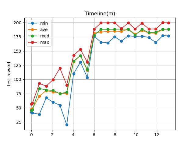
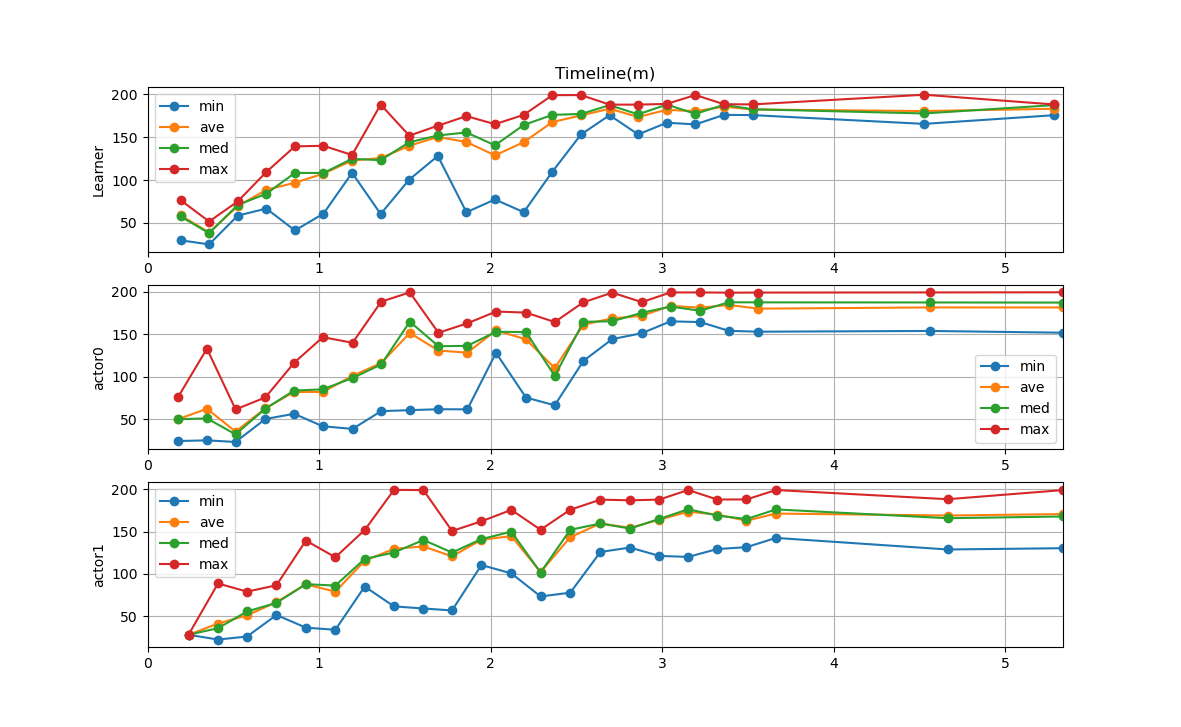
投稿日：2020-05-15T20:39:12+09:00

Inkbird IBS-TH1の値をRaspberryPiでロギング

はじめに

本記事は、Omron環境センサ（BAG型）の記事と同内容を、
低価格なInkbird IBS-TH1で実施した記事です。
前回使用したminiは電池の持ちが悪かったので、単4電池の本製品で持久性アップを狙いました。

Inkbirdとは？

様々な家庭用IoTセンサを作っている中国・深圳のメーカーです。
低価格（3000円くらい）でスマホアプリやAPIでのデータ取得等、一通りの機能がそろっている事が魅力です。

今回は、温度＋湿度センサ搭載の
Inkbird IBS-TH1

で、ロギングを実施します。

必要なもの

・RaspberryPi（今回はPi3Model Bを使用）
・Python実行環境（今回はpyenvでPython3.7.6使用）
・Inkbird IBS-TH1（プローブを外した状態で使用しています）

手順

①RaspberryPiとセンサのBluetooth接続確認
②センサの測定値をPythonで取得
③PythonからGASのAPIを叩いてスプレッドシートにデータ書き込み
④スクリプトの定期実行

こちらを参考にさせて頂きました。
https://qiita.com/bon_dentetsu/items/87ed6c65640b5ba11e5c
https://github.com/viyh/inkbird
https://github.com/sputnikdev/eclipse-smarthome-bluetooth-binding/issues/60

①RaspberrypiとセンサのBluetooth接続確認

センサの認識確認

・センサのセットアップ
センサに単4電池をセットします（蓋が取りずらいので注意してください）

・Bluetooth機器のスキャン
RaspberryPiで下記コマンドを実行
sudo hcitool lescan
LE Scan ...
AA:CC:EE:DD:55:77 sps
というように、「sps」という名前がでてきたら、これがセンサのMACアドレスです。
出てこなければ電池の接触やRaspberryPiのBluetooth有効を確認してください。
機種や設定によっては名前が「sps」ではないのかもしれないので、
その場合Inkbirdの公式アプリでMACアドレスを確認できます。

②センサの測定値をPythonで取得

bluepyでの認識確認

bluepyは、PythonでBluetooth Low Energy(BLE)にアクセスするためのライブラリです（クラス定義）

・必要なパッケージのインストール
下記をインストールします
sudo install libglib2.0-dev
・bluepyのインストール

下記コマンドでpipでインストールします
pip install bluepy
・bluepyに権限を付与
スキャンにはbluepyにSudo権限を与える必要があります。

bluepyのインストールされているフォルダに移動し、
cd ~.pyenv/versions/3.7.6/lib/python3.7/site-packages/bluepy
※上記は、pyenvでPython3.7.6をインストールした場合。
環境により場所は異なるので注意

下記コマンドでbluepy-helperにSudo権限を付与する
sudo setcap 'cap_net_raw,cap_net_admin+eip' bluepy-helper
センサ値取得スクリプトの作成

センサ値取得のため、下記のスクリプトを作成します
inkbird_ibsth1_connect.py
from bluepy import btle
import struct

def get_ibsth1_data(macaddr):
    peripheral = btle.Peripheral(macaddr)
    characteristic = peripheral.readCharacteristic(0x28)
    (temp, humid, unknown1, unknown2, unknown3) = struct.unpack('<hhBBB', characteristic)
    sensorValue = {
            'Temperature': temp / 100,
            'Humidity': humid / 100,
            'unknown1': unknown1,
            'unknown2': unknown2,
            'unknown3': unknown3,
        }
    return sensorValue
Inkbird IBS-TH1 miniではハンドルが「0x002d」でしたが、今回は「0x28」なので注意してください。
bluepyのPeripheralクラスによる通信でデータを取得します。

なお、取得したcharacteristicデータは
・1～2バイト目：温度（0.01℃単位）
・3～4バイト目：湿度（0.01％単位）
ですが、5～7バイト目の内容が調べてもわからなかったので、
unknown1～3としてロギングして、正体を探ろうと思います。
（電池残量が取得できる事を目論んでいます）

メインスクリプトの作成

センサ値取得スクリプトを呼び出すため、メインスクリプトを作成します
inkbird_toSpreadSheet.py
from bluepy import btle
import inkbird_ibsth1_connect

######オムロン環境センサ（BAG型）の値取得######
PERIPHERAL_MAC_ADDRESS = '①で取得したMACアドレス'
sensorValue = inkbird_ibsth1_connect.get_ibsth1_data(PERIPHERAL_MAC_ADDRESS)

#試しに温度を表示
print(sensorValue['Temperature'])
コンソールから実行してみます
python inkbird_toSpreadSheet.py
25.49
これで、Pythonでセンサ測定値を取得することができました。

③PythonからGASのAPIを叩いてスプレッドシートにデータ書き込み

オムロン環境センサの記事ご参照ください

④スクリプトの定期実行

オムロン環境センサの記事ご参照ください

　 Tweet
Qiitaで続きを読む

投稿日：2020-05-15T20:33:07+09:00

ターミナルに現れる意図せぬ(base)を消そう【Condaの環境から抜ける】

これはなに

ターミナルの先頭に現れる(base)を消そうという記事

↑お前誰や

そもそもこれなに

Conda は Python のバージョン管理ツール¹です。
機械学習のライブラリ欲張りセットである Anaconda をインストールすると標準でついてきます。
(base) が出ている状態である、ということは Conda が提供する仮想環境に入っている状態です。
特に問題がなければそのままで構いませんが、「Conda 以外のバージョン管理ツール（ pipenv, poetry など)を使いたい」、「なんかよくわからないけど不安だから消したい」みたいな時には不便ですよね。

消そう

消します。

一時的に消す

ターミナルで以下のコマンドを実行します。
仮想環境から一時的に抜ける
$ conda deactivate
これで仮想環境から出て、忌むべき(base)を消し去れました。
しかし、ターミナルを再起動したらまた憎い(base)が再び現れるかもしれません。その場合は以下で対処します。

永続的に消す（復元可能）
仮想環境にデフォルトで入らないようにする
$ conda config --set auto_activate_base False
Conda の config を書き換えて、デフォルトで仮想環境に入らないように設定します。これで再起動しても現れないはず。

帰ってきて Conda

逆に戻るときは以下です。
仮想環境に入り直す
$ conda activate
バージョン管理ツール: ライブラリの導入や削除、またライブラリ同士の依存関係を管理するシステムのこと ↩

　 Tweet
Qiitaで続きを読む

投稿日：2020-05-15T19:29:11+09:00

FlaskとDjangoのJSONデータの受け取り方の違いにハマる

こんばんは、@0yanです。
今日はLINE WORKS版Trello BotのFlaskアプリを、LINE WORKS問い合わせ対応BotのDjangoアプリに統合する際、JSONデータの受け取り方の違いにハマった（ダサイ･･･）ので、しくじり先生的な感じで記事書きます。
※LINE WORKS版Trello Botの作成方法はこちら

Flaskの場合

data = request.json['key']で、辞書型の値として受け取れます。

具体例（Flaskの場合）

@app.route('/webhook', methods=['HEAD', 'POST'])
def comment_notification_to_talk_room():
    if request.method == 'HEAD':
        return '', 200
    elif request.method == 'POST':
        action_type = request.json['action']['display']['translationKey']  # ★ココ
        if action_type == 'action_comment_on_card':
            card_name = request.json['action']['data']['card']['name']
            user_name = request.json['action']['memberCreator']['fullName']
            comment = request.json['action']['data']['text']
            message = f'{user_name}さんがコメントしました。\n【カード】{card_name}\n【コメント】{comment}'
            talk_bot.send_text_message(send_text=message)
            return '', 200
    else:
        abort(400)

Djangoの場合

body = json.loads(request.body)のように、JSONから辞書型に変換する必要があります。

具体例（Djangoの場合）

def comment_notification_to_talk_room(request, bot_no, account_id=None, room_id=None):
    talk_bot = TalkBotApi(api_id, server_api_consumer_key, server_id, private_key, domain_id, bot_no)

    # リクエストボディをJSONから辞書型に変換、action_typeを取り出す
    body = json.loads(request.body)  # ★ココ
    action_type = body['action']['display']['translationKey']

    # TrelloのコメントをLINE WORKSトークルームに送信
    if action_type == 'action_comment_on_card':
        card_name = body['action']['data']['card']['name']
        user_name = body['action']['memberCreator']['fullName']
        comment = body['action']['data']['text']
        message = f'{user_name}さんがコメントしました。\n【カード】{card_name}\n【コメント】{comment}'
        if account_id is not None:
            talk_bot.send_text_message(send_text=message, account_id=account_id)
            logger.info(f'通知成功  accountID:{account_id}')
        elif room_id is not None:
            talk_bot.send_text_message(send_text=message, room_id=room_id)
            logger.info(f'通知成功  roomID:{room_id}')
        else:
            logger.error('accoutId, roomIdはどちらか一方を指定する必要があります。')

いやー、こんなくだらないことに数時間使ってしまうとは･･･。
この失敗が誰かの役に立つことを願っています。

　 Tweet
Qiitaで続きを読む

投稿日：2020-05-15T19:26:17+09:00

Django2系でform.is_valid()の結果が常にFalseになる事象の対応

事象と環境

事象

views.pyに書いたViewクラスのpostメソッドで、is_validを実行した。
WEBブラウザ上でどのような入力をした場合でも、is_validの結果がFalseになった。

forms.pyでバリデーションメソッドは実装していない。

以下にソースコードの抜粋を示す。
FormクラスにMetaクラスがあるが、今回の事象とは関係ない認識である。
views.py
class View(View):
    def post(self, request, *args, **kwargs):
        form = Form()
        is_valid = form.is_valid()
        print(is_valid)
        ...
forms.py
class Form(forms.ModelForm):
    class Meta:
        model = ExperimentResult
        fields = ("title", "comment",)
        widgets = {
            'title' : forms.TextInput(attrs={'class':'text_area'}),
            'comment' : forms.TextInput(attrs={'class':'text_area'})
        }
環境

実行環境はdjango2.2.12、python3.7、Windows10である。
※OS、pythonバージョンは関係ないと想定される。

原因

Formクラスをインスタンス化する際に、initメソッドの第一引数に"request"があることを想定している。

form=FormClass()と書いたときには、initメソッドに"request"が渡されない。そのため、"is_valid"メソッドを実行すると、"request"が渡されていないことで、バリデーションエラーが発生し、必ずFalseが帰ってくる。

対応

Formクラスをインスタンス化する際に引数としてdata=request.POSTを入れる。
※GETメソッドの場合はrequest.GETになると想定される。
views.py
class View(View):
    def post(self, request, *args, **kwargs):
        form = Form(data=request.POST)
        is_valid = form.is_valid()
        print(is_valid)
        ...
上記対応後、Trueが帰ってくることを確認した。

参考

https://stackoverflow.com/questions/20801452/django-form-is-valid-always-false

　 Tweet
Qiitaで続きを読む

投稿日：2020-05-15T18:47:08+09:00

Pythonのfor&配列を簡単に理解する（超初心者向け）

私は独学でPythonでAtCoderに参加しています。
そこで今日は、学び始めた人（過去の私みたいな人）がわからなくなるポイントであるforと配列の簡単な解説をしようと思います！
AtCoderのforを使った入力などの話も絡めて解説します。あくまで簡単な解説です。最低ここまで知ることができたらググり力（ググるときの語彙力）も身につきます、自分で色々な関数をその都度ググって、少しずつ覚えていってくださいね！
（私は駆け出し茶色コーダーで、短い記法などは得意ではないです。また万が一嘘を書いていたら教えて欲しいです＞＜）

for文ってなんだYo！

ふつうのかきかた
for i in range(3):
    print(i)
for文はこのような形をしています。range()のカッコの中の数字の回数、for文内部の処理が繰り返されます。
この中でいうiは、ループカウンタ変数と言って、（私もググってて今知りましたw名前はどうでもいいです）繰り返すごとに1ずつ増えていきます。

このコードの実行結果は、
0
1
2
となります。

ここで見てもらうとわかるように、一発目のループのiは0となっていますね。ここが後々すごく重要なポイントとなります。
0,1,2合わせて3回出力されているのがわかります。range(3)と書いたからですね。

はじめとおわりを決めておくかきかた
for i in range(1,3):
    print(i)
実はこんな書き方もあります。
これの出力結果は
1
2
です。上のコードと見比べてみれば決まりがわかると思います。

発展　〜for文を重ねる〜

for文は重ねて書くことができます。まあ今のところはへーふーんそーなんだ程度に見てください。
for i in range(2):
    for j in range(3):
        print(i,j)
出力結果
0 0
0 1
0 2
1 0
1 1
1 2
ちょっと頭がこんがらがると思いますが、慣れるといけます！
（ちなみにfor文をたくさん重ねると実行時間が多くかかります。）

配列ってなんなんデイ！

配列（list）はざっくり言うと複数の要素をまとめて収納できる変数みたいなものです。
yasai = ["にんじん","だいこん","ごぼう"]
のように、要素がカンマ区切りで全体を[]で囲まれてできています。この場合でいうと、yasaiは3つ部屋があるホテルだと思ってください。
普通ホテルのひとつひとつの部屋にはそれぞれ部屋番号がありますね。配列も同じです。

配列は一番前の要素から順に、0,1,2....と番号がついています。この番号をindexといいます。

もう一度言います！！一番前の要素の番号は0！！！
さっきのiと同じです。めちゃめちゃ大事なポイントなのでおさえましょう。

index指定をやってみよう
yasai = ["にんじん","だいこん","ごぼう"]
print(yasai[1])
また、このように配列名[数字]と書くことで、配列のその番号の要素を取得することができます。
このコードの実行結果、わかりますか？

「にんじん」だと思った方いませんか？違いますよ！
だいこん
一番前の要素の番号は0、絶対に間違えないようにしましょう。

配列の長さはlen！

配列の長さはlen(配列)で取得することができます。
yasai = ["にんじん","だいこん","ごぼう"]
print(len(yasai))
出力結果
3
これもよく使います。覚えておきましょう。

ここまでのことをふまえて

あなたはこんなコードが書けるようになりました。
yasai = ["にんじん","だいこん","ごぼう"]
for i in range(len(yasai)):
    print(yasai[i])
出力結果↓
にんじん
だいこん
ごぼう
どうですか！ここまで理解できれば、C問題が解けるようになってきてます。わからなかったらもう一度上をよんでみてください。

for文を使った入力、配列の入力をやってみイェイ！（AtCoder）

AtCoderだとだいたいC問題あたりからforを使った入力が出てくると思います。
例えばこんな感じのやつです↓

C - Peaks

※問題の解き方の解説はしません。入力のやり方だけ説明します。

入力欄を見るとこういう風になっています。

意味がわからないかもしれません。私も最初は意味がわかりませんでした。特に添字。
でも上を理解できたならすぐわかるようになります。
N,M = map(int,input().split())
H = list(map(int,input().split()))
for i in range(M):
    A,B = map(int,input().split())
ジャジャーン。
listの入力の仕方はいつものmap()入力にlist()をかぶせるだけです。
下のfor文ではM回ループを回し、M回ぶんA、Bを入力しています。

ここでわかると思いますが、Pythonは配列の入力をするときに配列の長さの指定がいらないので、Nは入力の時にMのようには使わないです。かんたんですね。

入力の指定（灰色の画像参照）より、N == len(H)が成り立っています。

みんな大嫌い配列外参照　〜エラーメッセージを読もう〜

初学者がもっともイライラするエラーのひとつに、配列外参照があります。
yasai = ["にんじん","だいこん","ごぼう"]
print(yasai[3])
さて、こんなコードがあります。何が出力されるかわかりますか？

「ごぼう」と思った人が万が一にもいたらもう一度上のページに戻って私の言葉を心に刻みましょう。

答えは、「何も出力されない」です。エラーメッセージが出ます。
Traceback (most recent call last):
  File "Main.py", line 2, in <module>
    print(yasai[3])
IndexError: list index out of range
こんなエラーが出ます。

英語できなくても、落ち着いて読めば全然難しくありません。

line 2から、2行目のコードがおかしいのだとわかります。
IndexError: list index out of rangeを見てください。これが私がもっとも嫌いな（よく出してしまう）インデックスエラー、配列外参照です。

つまり、このエラーメッセージを読めば、「2行目のコードprint(yasai[3])のインデックスが配列の外を参照しているよ」ということがわかるわけです！

この配列外参照はパッと見単純なことのように見えますが、コードが複雑になってくると恐怖の配列外参照オンパレード地獄になります。気をつけましょう。

最後に

C問題まである程度の速さで解けるようになれば、確実に茶色コーダーを目指せます！
Pythonは書くコードが短くてよく基本速解きに向いた言語だし、何より読みやすいので、猛烈に時間かかった私がいうのもアレですが、茶色までなら比較的すぐ行けるかもしれません。

実行時間（競プロには実行時間の制限があります、なるべく効率の良いコードを書こうね〜ってことですね、詳しくはwebで）がいちばんの問題なのですが、計算量の色々は慣れればある程度までは体感でわかると思います。

頑張ってください！

　 Tweet
Qiitaで続きを読む

投稿日：2020-05-15T18:40:15+09:00

hogehoge

　 Tweet
Qiitaで続きを読む

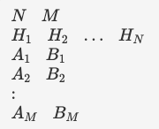
投稿日：2020-05-15T18:33:46+09:00

ALBのデフォルトセキュリティグループをCDKからいじりたいんだって

概要

CDKでALB with Fargateを作るとSecurityGroupがフル開放されちゃいます
開発環境だったり、内部のサービスであれば、セキュリティを考えてIPを絞りたいと思うのですが、CDKだと追加は簡単だけど削除が難しかったので、その方法の共有です

手順

フルオープンSG作成

まずは変更対象のSecurityGroupを作成します

alb_sg=ec2.SecurityGroup(self, "alb-sg",
    vpc=ivpc,
    description="alb sg"
)

次にそのSecurityGroupを利用したALBを作成します

ecs_alb=elasticloadbalancingv2.ApplicationLoadBalancer(self, "alb",
    security_group=alb_sg,
    vpc=ivpc,
    internet_facing=True,
    load_balancer_name="ecs-alb"
)

そしてecs_patternsを使ってFargateServiceを作ります

fargate_service = ecs_patterns.ApplicationLoadBalancedFargateService(self, "service",
    cluster=cluster,
    task_definition=task,
    load_balancer=ecs_alb,
    cloud_map_options = ecs.CloudMapOptions(
        name = 'hoge'
    )
)

実行すると下記のように80ポートがフルオープンしたSecurityGroupが作成されることが分かります
（SecurityGroupの部分のみ抜き出してます）

$ cdk diff ecs
Stack ecs
Security Group Changes
┌───┬───────────────────────────────────────────────────────┬─────┬──────────┬────────────────────────────────┐
│   │ Group                                                 │ Dir │ Protocol │ Peer                           │
├───┼───────────────────────────────────────────────────────┼─────┼──────────┼────────────────────────────────┤
│ + │ ${prod-alb-sg.GroupId}                        │ In  │ TCP 80   │ Everyone (IPv4)                │
└───┴───────────────────────────────────────────────────────┴─────┴──────────┴────────────────────────────────┘
Resources
[~] AWS::EC2::SecurityGroup prod-alb-sg prodmonitoralbsg0D94D960 
 └─ [+] SecurityGroupIngress
     └─ [{"CidrIp":"0.0.0.0/0","Description":"Allow from anyone on port 80","FromPort":80,"IpProtocol":"tcp","ToPort":80}]

SGの上書き

node.default_child.add_override で上書きできるので、キーを指定して上書きします
下記２個を指定していて、フル開放されている1つしかルールが追加されてないので０番目を指定してます

Properties.SecurityGroupIngress.0.CidrIp
Properties.SecurityGroupIngress.0.Description

alb_sg.node.default_child.add_override(
    "Properties.SecurityGroupIngress.0.CidrIp",
    "1.1.1.1/32"
)
alb_sg.node.default_child.add_override(
    "Properties.SecurityGroupIngress.0.Description",
    "Google"
)

実行すると、デフォルトのTCP80 allow Everyoneが消えて指定したIPに変わります

$ SYSTEM_ENV=prod cdk diff ecs
Stack ecs
Security Group Changes
┌───┬────────────────────────────────┬─────┬──────────┬─────────────────┐
│   │ Group                          │ Dir │ Protocol │ Peer            │
├───┼────────────────────────────────┼─────┼──────────┼─────────────────┤
│ - │ ${prod-alb-sg.GroupId} │ In  │ TCP 80   │ Everyone (IPv4) │
├───┼────────────────────────────────┼─────┼──────────┼─────────────────┤
│ + │ ${prod-alb-sg.GroupId} │ In  │ TCP 80   │ 1.1.1.1/32 │
└───┴────────────────────────────────┴─────┴──────────┴─────────────────┘
(NOTE: There may be security-related changes not in this list. See https://github.com/aws/aws-cdk/issues/1299)

Resources
[~] AWS::EC2::SecurityGroup prod-alb-sg prodmonitoralbsg0D94D960 
 └─ [~] SecurityGroupIngress
     └─ @@ -1,7 +1,7 @@
        [ ] [
        [ ]   {
        [-]     "CidrIp": "0.0.0.0/0",
        [-]     "Description": "Allow from anyone on port 80",
        [+]     "CidrIp": "1.1.1.1/32",
        [+]     "Description": "Google",
        [ ]     "FromPort": 80,
        [ ]     "IpProtocol": "tcp",
        [ ]     "ToPort": 80

以上がCDKからALBデフォルトSGのいじり方でした

参考

　 Tweet
Qiitaで続きを読む

投稿日：2020-05-15T18:27:16+09:00

Statsmodelsによるディッキーフラー検定

分析の対象となる時系列データがランダムウォークにしたがうのかどうかを調べる方法としてディッキーフラー検定があります。しかし、検出力が低いとよく指摘されています。そこで少し調べてみようと思います。

DF検定に移る前に

確率論では、確率的ドリフトは、確率過程の平均値の変化のことです。同じような概念でドリフト率があります。これは平均が変化する率のことです。

長期にわたる事象に関する長期的な研究では、時系列の特性を、トレンド成分、周期成分、および確率的な成分（確率的ドリフト）に分解して概念化することがよくあります。周期的および確率的ドリフトの成分は、自己相関分析と傾向(トレンド)の階差を取ることで識別されます。自己相関分析は、適合モデルの正しい位相を特定するのに役立ち、階差を繰り返すことは確率的ドリフト成分をホワイトノイズに変換します。

トレンド定常

トレンド定常過程$y_t$は、$y_t = f（t）+ u_t$に従います。ここで、tは時間、fは決定論的関数、$u_t$は長期的な平均値がゼロとなる定常確率変数です。この場合、確率的項は定常的であり、したがって確率的ドリフトはありません。確定的な成分f(t)は長期的に一定に保たれる平均値を持ちませんが、時系列自体がドリフトする可能性があります。この確定的ドリフトは、tで$y_t$を回帰し、定常な残差がえられれば、データから削除して求めることができます。

階差定常

対照的に、単位根（定常）過程は、$y_t = y_ {t-1} + c + u_t$に従います。$u_t$は長期的にはゼロとなる平均値をもつ定常確率変数です。ここでcは非確率的ドリフトパラメーターです。ランダムショック$u_t$がなくても、yの平均は期間ごとにcだけ変化します。この非定常性は1次の階差を取ることでデータから削除できます。階差された変数$z_t = y_t-y_{t-1}=c+u_t$はcの長期的に一定となる平均値を持ち、したがってこの平均値にドリフトはありません。つぎにc = 0として考えてみます。この単位根過程は、$y_t = y_ {t-1} + c + u_t$です。$u_t$は定常過程ですが、その確率的なショック$u_t$の存在により、ドリフト、特に確率論的ドリフトが$y_t$に生じます。一度発生したゼロ以外の値uは同じ期間のyに組み込まれます。これは、1期間後にyの1期間遅れの値になり、次の期のy値にも影響します。 yは次々に新しいy値に影響を与えます。したがって、最初のショックがyに影響した後、その値はyの平均に永久に組み込まれるため、確率的なドリフトが生じるのです。ですからこのドリフトも、最初にyを微分してドリフトしないzを取得することで除くことができます。この確率的ドリフトは$c\ne0$でも生じます。ですから$y_t = y_ {t-1} + c + u_t$でも生じます。cは非確率的ドリフトパラメーターと説明しました。なぜ確定的なドリフトではないのでしょうか？実は、$c+u_t$から生じるドリフトは確率過程の一部です。

numpy.random.normal

numpyのリファレンスから

numpy.random.normal(loc=0.0, scale=1.0, size=None)

loc float or array_like of floats: 分布の平均値

scalefloat or array_like of floats：分布の標準偏差

です。ここでlocの意味を考えてみます。この分布から生成される標本の平均値は$N(μ,σ^2/n)$に近似的に従います。その仕組みをみてみましょう。あえてloc=1,scale=1.0とします。n=2としてその標本平均と標準偏差を求めてみました。ただし、計算方法は2つです。1つは
$z_t$の平均と標準偏差を求めます。
もう1つは
それぞれの観測値$z_t$から１を引きその標本の平均と標準偏差を求めます。そしてその標本平均に1を足します。
import numpy as np
import matplotlib.pyplot as plt

s = np.random.normal(1, 1, 2)
print(np.mean(s),np.std(s))
o=np.ones(len(s))
Print(np.mean(s-o)+1,np.std(s-o))

# 0.9255104221128653 0.5256849930003175
# 0.9255104221128653 0.5256849930003175 # 標本から１を引いて、その平均値に１を足した。
結果は同じになりました。しかし、標本平均と標準偏差はともに１ではありません。そこでn=2とn=100の場合について10000回データを生成してその結果がどうなるかを見てみましょう。

階差定常過程の標本の算術平均の分布

階差された変数$z_t = y_t-y_{t-1}=c+u_t$はcの長期的に一定となる平均値を持ちます。その標本平均はnが大きければ、$N(μ,σ^2/n)$に近似的に従います。したがって、平均値は一定ではありません。しかし、この場合には平均値にドリフトはありません。長期的に一定となる平均値をもちます。
m1=[]
trial=1000000
for i in range(trial):
    s = np.random.normal(1, 1, 2)
    m1.append(np.mean(s))
m2=[]
for i in range(trial):
    s = np.random.normal(1, 1, 100)
    m2.append(np.mean(s))
bins=np.linspace(np.min(s),np.max(s),1000)
plt.hist(m1,bins=bins,label='n=2')
plt.hist(m2,bins=bins,label='n=100',alpha=0.5)
plt.legend()
plt.show()
標本平均も標準偏差も分布を形成し、一意には定まりません。一意に定まるためにはnはもっともっと大きくする必要があります。したがって、時系列の特性を、トレンド成分、周期成分、および確率的な成分（確率的ドリフト）に分解して概念化しますが、確率的ドリフトとドリフト率の扱いには注意が必要です。

単位根過程では確率的ドリフトが発生します。もし、確定的なドリフト率があったとしてもそれは識別が不可能です。

単位根過程のyの分布

単位根過程では標本の数が増えるにつれて標準偏差は大きくなっていきます。標本の大きさがnのyの平均値はc=0ではゼロですが、標準偏差$\sqrt{n \cdot \sigma^2}$が大きくなった分だけ、その分布は広がります。
m1=[]
trial=1000000
for i in range(trial):
    s = np.cumsum(np.random.normal(0, 1, 2))
    m1.append(s[-1])
m2=[]
for i in range(trial):
    s = np.cumsum(np.random.normal(0, 1, 100))
    m2.append(s[-1])
bins=np.linspace(np.min(m2),np.max(m2),1000)
plt.hist(m1,bins=bins,label='n=2')
plt.hist(m2,bins=bins,label='n=100',alpha=0.5)
plt.legend()
plt.show()
先ほどとは異なる分布になりました。標本の大きさが大きいほうの分布の広がりが大きくなります。ためしに１つのsの系列をプロットして見ましょう。
plt.plot(s)
この場合、階段的にそれぞれの標本のレベルが変化していきます。この変化は確率的なショック$u_t$によるものです。それが加算されていったものがプロットされています。確率的ドリフトの系列がプロットされています。これが大きなトレンドを形成することがあります。それはn=100の分布図でいえば両端の領域に相当します。どの範囲かはトレンドの定義によります。そのトレンドは確率的トレンドです。これはトレンド定常性がつくる確定的トレンドと明確に区別されます。

検出力(statsmodelsによる統計的仮説検定入門)

仮説検定では帰無仮説と対立仮説を立てます。帰無仮説は母数で構成します。母数は一般的には未知なので推定値を用いることもあります。標本はこの母集団から抽出されたものとして扱います。つぎの図では、その母数の分布を青い点線で示しています。標本からはその統計量の標本分布が得られます。この2つを比べます。2つの分布が近ければ、この2つの分布を違うと判断するのが難しく、離れていれば違うと判断できます。この判断を有意水準を用いて行うことができます。有意水準$\alpha$は母集団の右端の面積のことです。10%,5%などが用いられます。青い分布の青い垂直の線の右側の面積です。p値は母集団(母数の分布)から標本(統計量)が得られる確率を示します。この値が判断基準である有意水準より小さければ、標本(統計量)は母集団(母数)とは異なる分布から得られたと判断します。検出力$\beta$とは青い垂直の線の橙の分布の右側の面積のことです。理想的には$\beta$の部分が大きければ帰無仮説を棄却した時に対立仮説が正しい確率が大きくなります。この$\beta$を大きくするためには2つの分布が大きく離れている、または分布の中心の位置が大きく異なることが考えられます。もう1つは標本の大きさが大きいことです。そうすれば分布の形状は狭くなり２つの直線を比べることになります。

Dicky-fuller検定

単純なAR(1)過程を
$ y_t= \rho y_{t-1}+u_t$
とし、両辺から$y_{t-1}$を差し引いて
$y_t-y_{t-1}=(\rho-1)y_{t-1}+u_t$
とします。$\delta=\rho-1$として、帰無仮説はARモデルに単位根が存在するとします。
$H_0$:$\delta=0$
$H_1$: $\delta<0$
となります。

3つのタイプがあります。
1)ドリフト無しランダムウォーク
$\Delta y_t=\delta y_{t-1}+u_t$
2) ドリフト付きランダムウォーク
$\Delta y_t=c+\delta y_{t-1}+u_t$
3) ドリフト付きランダムウォーク＋時間トレンド
$\Delta y_t=c+c\cdot t+\delta y_{t-1}+u_t$

1次の自己回帰過程

1次の自己回帰過程はつぎに様に書き換えることができます。
$x_1=ρ\cdot x_0+y_1+e_1$
$x_2=ρ\cdot x_1+y_2+e_2$
$x_3=ρ\cdot x_2+y_3+e_3$

$x_2=ρ\cdot (ρ\cdot x_0+y_1+e_1)+e2=ρ^2\cdot x_0+ρ\cdot (y_1+e1)+e2$
$x_3=ρ\cdot (ρ\cdot ρ\cdot x_0+ρ\cdot (y_1e_1)+e_2)+e_3$
$=ρ^3x_0+ρ^2\cdot (y_1+e_1)+ρ\cdot (y_2+e_2)+y_3+e_3$
ここで$y_i=c+d\cdot i$

ランダムウォーク過程

単位根過程はつぎのように書き換えることができます。
$x_1=x_0+c+e_1$
$x_2=x_1+c+e_2$
$x_3=x_2+c+e_3$

$x_2=(x0+c+e_1)+c+e2=x_0+c+e1+c+e2$
$x_3=(x0+c+e_1+c+e_2)+e_3=x_0+e_1+e_2+e_3+3 \cdot c$
# 初期化
import numpy as np
import statsmodels.api as sm
import matplotlib.pyplot as plt
from scipy.stats import norm
from statsmodels.tsa.stattools import adfuller
#np.random.seed(0)
# AR(1)過程の生成
# x0は価格の初期値
# nsampleは1回の試行の期間の数
# rho=1: random walk
## c=c1-rho はドリフト、c1=1のときはドリフト無しランダムウォーク　dは確定的トレンド
# rho<1で1次の自己回帰モデル
## x0とcとdの効果は時間の経過とともに消滅 
def ar1(rho,x0,c1,d,sigma,nsample):
    e = np.random.normal(size=nsample)#random variable
    rhoo=np.array([rho ** num for num in range(nsample)]) #effects of rho
    rhoo_0=np.array([rho**(num+1) for num in range(nsample)]) #effects of rho
    t=np.arange(nsample) #deterministic trend
    one=np.ones(nsample) #effect of x0
    x00=x0*one*rhoo_0 #effect of rho to x0
    c=c1-rho # constant of autoregressive mdoel
    c0=np.cumsum(c*one*rhoo) #effect of rho to c
    d0=(d*t*rhoo) # effect of rho to determinist trend
    y=np.cumsum(rhoo*e*sigma)+x00+c0+d0
    return y
# Dicky-Fuller検定のテスト
def adfcheck(a0,mu,sigma,nsample,trial):
    prw=0
    prwc=0
    prwct=0
    for i in range(trial):
        y=ar1(a0,1,mu,sigma,nsample)
        rw=sm.tsa.adfuller(y,maxlag=0,regression='nc')[1]
        rwc=sm.tsa.adfuller(y,maxlag=0,regression='c')[1]
        rwct=sm.tsa.adfuller(y,maxlag=0,regression='ct')[1]
        if rw>0.05:
            prw+=1
        if rwc>0.05:
            prwc+=1
        if rwct>0.05:
            prwct+=1
    print('nsample',nsample,prw/trial,prwc/trial,prwct/trial)
ドリフト無しランダムウォーク
rho=1
c1=1
c1=(c1-1)/250+1
d=0
d=d/250
sigma=0.4/np.sqrt(250)
trial=10000    
for i in [7,20,250]:
    adfcheck(rho,x0,c1,d,sigma,i,trial)

# nsample 7 0.9423 0.8837 0.8489
# nsample 20 0.9578 0.9361 0.9231
# nsample 250 0.9545 0.9476 0.9476
ドリフト付きランダムウォーク
rho=1
c1=1.1
c1=(c1-1)/250+1
d=0
d=d/250
sigma=0.4/np.sqrt(250)
trial=10000    
for i in [7,20,250]:
    adfcheck(rho,x0,c1,d,sigma,i,trial)

# nsample 7 0.9466 0.8895 0.8564
# nsample 20 0.9697 0.9316 0.9196
# nsample 250 0.9734 0.9492 0.9447
ランダムウォーク+ドリフト+確定的トレンド
rho=1
c1=1.1
c1=(c1-1)/250+1
d=0.9
d=d/250
sigma=0.4/np.sqrt(250)
trial=10000    
for i in [7,20,250]:
    adfcheck(rho,x0,c1,d,sigma,i,trial)

# nsample 7 0.9719 0.8864 0.8578
# nsample 20 0.9935 0.943 0.9229
# nsample 250 1.0 0.9817 0.944
ドリフト無しAR(1)モデル
rho=0.99
c1=rho
#c1=(c1-1)/250+1
d=0
d=d/250
sigma=0.4/np.sqrt(250)
trial=10000    
for i in [7,20,250]:
    adfcheck(rho,x0,c1,d,sigma,i,trial)

# nsample 7 0.7586 0.8972 0.8509
# nsample 20 0.5476 0.9479 0.909
# nsample 250 0.0004 0.2365 0.8084
ドリフト付きAR(1)モデル
rho=0.93
c1=1.1
c1=(c1-1)/250+1
d=0
d=d/250
sigma=0.4/np.sqrt(250)
trial=10000    
for i in [7,20,250]:
    adfcheck(rho,x0,c1,d,sigma,i,trial)

# nsample 7 0.9465 0.8474 0.8172
# nsample 20 0.967 0.7771 0.806
# nsample 250 0.973 0.0288 0.0644
AR(1)モデル+ドリフト+確定的トレンド
rho=0.90
c1=1.1
c1=(c1-1)/250+1
d=1
d=d/250
sigma=0.4/np.sqrt(250)
trial=10000    
for i in [7,20,250]:
    adfcheck(rho,x0,c1,d,sigma,i,trial)

# nsample 7 0.9694 0.8162 0.8
# nsample 20 0.9775 0.6663 0.7175
# nsample 250 0.9667 0.0316 0.055
正しい仕様もモデルを使うこと、標本の大きさは大きいほうが良いこと、そして帰無仮説を棄却するときにはρは１から離れていたほうが良いことが分かる。

ノイズの影響について

コーシー分布を使ってファットテイルのノイズを発生させそれを使って時系列を生成した時にどのような影響が出るかを調べてみます。
ノイズの分布をみます。
from scipy.stats import cauchy
trial=1000000
m1=[]
for i in range(trial):
    s = np.random.normal(0, 1, 250)
    m1.append(np.mean(s))
m2=[]
for i in range(trial):
    s=[]
    i=1
    while i<=250:
        s0 = (cauchy.rvs(0,1,1))
        if abs(s0)<10:
            s.append(s0)
            i+=1
    m2.append(np.mean(s))
bins=np.linspace(np.min(m2),np.max(m2),1000)
plt.hist(m1,bins=bins,label='normal')
plt.hist(m2,bins=bins,label='abs(cauchy) <10',alpha=0.5)
plt.legend()
plt.show()
ノイズの和の分布をみます。
from scipy.stats import cauchy
m1=[]
trial=1000000
for i in range(trial):
    s = np.cumsum(np.random.normal(0, 1, 250))
    m1.append(s[-1])
m2=[]
for i in range(trial):
    s=[]
    i=1
    while i<=250:
        s0 = (cauchy.rvs(0,1,1))
        if abs(s0)<10:
            s.append(s0)
            i+=1
    m2.append(np.cumsum(s)[-1])
bins=np.linspace(np.min(m2),np.max(m2),1000)
plt.hist(m1,bins=bins,label='normal')
plt.hist(m2,bins=bins,label='cauchy',alpha=0.5)
plt.legend()
plt.show()
def ar1_c(rho,x0,c1,d,sigma,nsample):
    e = cauchy.rvs(loc=0,scale=1,size=nsample)    
    rhoo=np.array([rho ** num for num in range(nsample)]) #effects of rho
    rhoo_0=np.array([rho**(num+1) for num in range(nsample)]) #effects of rho
    t=np.arange(nsample) #deterministic trend
    one=np.ones(nsample) #effect of x0
    x00=x0*one*rhoo_0 #effect of rho to x0
    c=c1-rho # constant of autoregressive mdoel
    c0=np.cumsum(c*one*rhoo) #effect of rho to c
    d0=(d*t*rhoo) # effect of rho to determinist trend
    y=np.cumsum(rhoo*e*sigma)+x00+c0+d0
    return y
def adfcheck_c(rho,x0,c1,d,sigma,nsample,trial):
    prw=0
    prwc=0
    prwct=0
    for i in range(trial):
        y=ar1_c(rho,x0,c1,d,sigma,nsample)
        rw=sm.tsa.adfuller(y,maxlag=0,regression='nc')[1]
        rwc=sm.tsa.adfuller(y,maxlag=0,regression='c')[1]
        rwct=sm.tsa.adfuller(y,maxlag=0,regression='ct')[1]
        if rw>0.05:
            prw+=1
        if rwc>0.05:
            prwc+=1
        if rwct>0.05:
            prwct+=1
    print('nsample',nsample,prw/trial,prwc/trial,prwct/trial)
rho=0.90
c1=1.1
c1=(c1-1)/250+1
d=1
d=d/250
sigma=0.4/np.sqrt(250)
trial=10000    
for i in [7,20,250]:
    adfcheck_c(rho,x0,c1,d,sigma,i,trial)

# nsample 7 0.9581 0.8267 0.8128
# nsample 20 0.9468 0.8 0.847
# nsample 250 0.8838 0.0718 0.1461
ファットテイルの影響で帰無仮説の棄却が減っています。

参考

Campbell, J. Y.; Perron, P. (1991). "Pitfalls and Opportunities: What Macroeconomists Should Know about Unit Roots"

Stock J. Unit Roots, Structural Breaks, and Trends. In: Engle R, McFadden D Handbook of Econometrics. Amsterdam: Elsevier ; 1994. pp. 2740-2843.

MacKinnon, J.G. 2010. “Critical Values for Cointegration Tests.” Queen’s University, Dept of Economics, Working Papers.

statsmodels.tsa.stattools.adfuller

単位根

ディッキー–フラー検定

Stochastic drift

http://web.econ.ku.dk/metrics/Econometrics2_05_II/Slides/08_unitroottests_2pp.pdf

　 Tweet
Qiitaで続きを読む

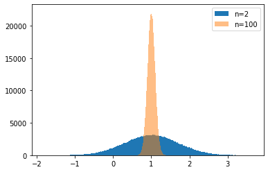
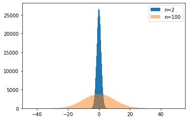
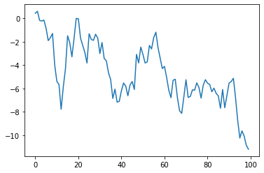
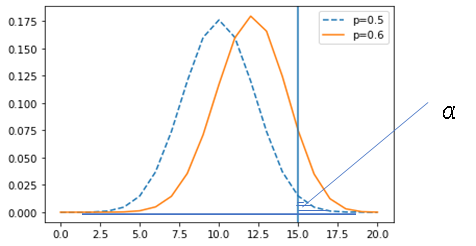
投稿日：2020-05-15T18:22:12+09:00

Linux & Pythonで自分自身のピークのメモリ使用量を取る

結論

いろいろ調べたのですが、これよりマシな方法が見つかりませんでした。
/procファイルシステムを使っているので、サポートしているプラットフォーム(Linux等)でしか動きません。
import os
import re

def peak_memory():
    pid = os.getpid()
    with open(f'/proc/{pid}/status') as f:
        # "VmHWM:    862168 kB" の形式になっている行を抜き出す
        for line in f:
            if not line.startswith('VmHWM:'):
                continue
            return int(re.search('[0-9]+', line)[0])
    raise ValueError('Not Found')
なぜピーク使用量か?

とある関数の内部で、一時的にメモリ使用量がハネ上がる現象が起きました。

その関数をプロファイリングしてメモリ使用量がハネ上がっている箇所を突き止めたいのであればmemory-profilerを使うのが良いかと思います。
今回、どこで増えるかは分かっていて、増えるのは仕方ないが、具体的にどれくらい増えるのかを調べたかったので、ピーク使用量を知る必要がありました。

ピーク使用量を使わないとどうなるか。

現在のメモリ使用量であればpsutilで取れます。このへんを参照。

ですが、ピークではないので、例えばこういうコードのとき
現在の使用メモリを取る
import psutil

def f():
    a = [0] * 20000000

print(psutil.Process().memory_full_info())
f()
print(psutil.Process().memory_full_info())
以下のような結果になります。
あんまり変わらない
pfullmem(rss=12406784, vms=18395136, shared=6369280, text=4096, lib=0, data=6225920, dirty=0, uss=8134656, pss=9319424, swap=0)
pfullmem(rss=12619776, vms=18354176, shared=6385664, text=4096, lib=0, data=6184960, dirty=0, uss=8253440, pss=9438208, swap=0)
f()の中ではメモリをいっぱい使っているのですが、外では使っていないので、外からでは分からないんですね。
fの中でも取ってみる
import psutil

def f():
    a = [0] * 20000000
    print('inner: ', psutil.Process().memory_full_info())

print('before:', psutil.Process().memory_full_info())
f()
print('after: ', psutil.Process().memory_full_info())
この場合、以下のようになります。
真ん中だけいっぱい使っている
before: pfullmem(rss=12476416, vms=18395136, shared=6443008, text=4096, lib=0, data=6225920, dirty=0, uss=8179712, pss=9407488, swap=0)
inner:  pfullmem(rss=172519424, vms=178356224, shared=6520832, text=4096, lib=0, data=166187008, dirty=0, uss=168300544, pss=169528320, swap=0)
after:  pfullmem(rss=12754944, vms=18354176, shared=6520832, text=4096, lib=0, data=6184960, dirty=0, uss=8298496, pss=9526272, swap=0)
メモリを使っていそうなところに、ピンポイントでメモリ使用量を取るコードを入れられるなら、それでいいんですが、そうしたくなかったわけです。

今回の方法ではどうなったか?
ピーク使用量を取る
import os
import re

def peak_memory():
    pid = os.getpid()
    with open(f'/proc/{pid}/status') as f:
        for line in f:
            if not line.startswith('VmHWM:'):
                continue
            return int(re.search('[0-9]+', line)[0])
    raise ValueError('Not Found')

def f():
    a = [0] * 20000000

print('before:', peak_memory(), 'KB')
f()
print('after: ', peak_memory(), 'KB')
結果、こうなりました。
afterで増えてる
before: 9072 KB
after:  165532 KB
めでたしめでたし。

参考文献

Linux プログラムのメモリ消費量を測る

コードについて

本記事に掲載されたコードを、自身・自社が開発されているPythonスクリプトに利用いただくのはご自由にどうぞ。

　 Tweet
Qiitaで続きを読む

投稿日：2020-05-15T17:57:04+09:00

Nuxt&Django REST FrameworkでCRUD PUT,DELETE編

概要

フロント:Nuxt
バックエンド:Django REST Framework（以下DRF）
で新しいプロジェクトなどを立ち上げた時に設定などをいちいち調べるのがめんどくさくなったため、まとめておきます。

ただ、設定ファイルだけを書くのでは個人的に記事として物足りない。

なので、ついでに基本的な操作であるAPIを叩いてCRUDを行い、会員登録を実装するところまで書く予定です。
なお、今回はDBはSQLiteを使います。PostgreSQLやMySQLなど他のRDBが使いたい場合はDRF側のDBの設定を書きかえるだけなので、そちらの設定は各自よろしくお願いいたします。

ひとまずこの記事では、NuxtからDRFで作ったAPIを叩いてデータベースの内容をアップデート、及びデリートするところまでです。

ソースコードはこちらにあるのでわからないところは適宜見てください。

また、Twitterかこの記事のコメント欄でわからないところを聞いていただけると答えられます。

前回
Nuxt&Django REST FrameworkでCRUD POST編

更新箇所

バックエンド

前回と同じようにviewとurlを追加します。

views.py

# 商品を編集・削除するためのview
class ItemEditView(generics.RetrieveUpdateDestroyAPIView):
    serializer_class = ItemSerializer
    queryset = Item.objects.all()

前回触れなかったのですが、私は使いやすいのでgenericsのviewを使っています。

今回使っているgenerics.RetrieveUpdateDestroyAPIViewは情報をGET、PUT、DELETEすることのできるviewです。
このviewを使う場面としては、今回のような商品の編集と削除画面を一つにしたいときでしょう。
なお、今回は編集する時にどこを変えるのかわかりやすいように元の登録されているデータを表示するためにGETもできるこちらを使っています。

viewの使い方や一覧等はこちらを見てください。

urls.py

.....
path('items/<int:pk>/edit',ItemEditView.as_view()),

前回もそうでしたが、これで設定は完了です。

http://localhost:8000/api/items/1/edit

にアクセスしてみましょう。

以上のようにidが1の商品の情報を表示し、かつPUTもDELETEもできるようになっていますね。

ではフロントエンドに移りましょう。

フロントエンド

今回は_idフォルダの中にedit.vueを作ります。

_id/edit.vue

<template>
<v-card
    light
    :loading="isUpdating"
  >
    <div id="app">
    <v-app id="inspire">
    <v-container>
    <div class="col-12 text-center my-3">
        <h3 class="mb-3 display-4 text-uppercase">
          {{ item.name }}
        </h3>
      </div>
      <div class="col-md-6 mb-4">
        <img
          class="img-fluid"
          style="width: 400px; border-radius: 10px; box-shadow: 0 1rem 1rem rgba(0,0,0,.7);"
          :src="item.image"
          alt
        >
      </div>
    <div class="col-md-6">
        <div class="item-details">
          <h4>カテゴリー</h4>
          <p>{{ item.category }}</p>
          <h4>値段</h4>
          <p>{{ item.price }}</p>
          <h4>説明</h4>
          <p>{{ item.description }}</p>
          </div>
          </div>
          </v-container>
    <v-form @submit.prevent="editItem">
      <v-container>
        <v-row>
          <v-col
            cols="12"
            md="4"
          >
            <v-text-field
              v-model="item.name"
              label="商品名"
              required
            ></v-text-field>
          </v-col>

          <v-col
            cols="12"
            md="4"
          >
            <v-text-field
              v-model="item.category"
              :counter="10"
              label="カテゴリー"
              required
            ></v-text-field>
          </v-col>

          <v-col
            cols="12"
            md="4"
          >
            <v-text-field
              v-model="item.price"
              label="値段"
              required
            ></v-text-field>
          </v-col>

          <v-col
            cols="12"
            md="4"
          >
            <v-text-field
              v-model="item.description"
              label="商品説明"
              required
            ></v-text-field>
          </v-col>
          <v-col
            cols="12"
            md="4"
          >
           <v-file-input
           v-model="item.image"
           label="商品画像"
           filled
           prepend-icon="mdi-camera"
           ></v-file-input>
          </v-col>
          <v-card-actions>
      <v-spacer />
      <v-btn
        class="btn-primary"
        :loading="isUpdating"
        color="primary"
        depressed
        @click="isUpdating = true"
        type="submit"
      >
        <v-icon left>
          mdi-post
        </v-icon>
        商品を更新
      </v-btn>
    </v-card-actions>
        </v-row>
      </v-container>
    </v-form>
    <v-form @submit.prevent="deleteItem">
    <button class="btn btn-sm btn-danger">
          削除
    </button>
    </v-form>
  </v-app>
</div>
</v-card>
</template>

<script>
export default {
    async asyncData ({ $axios, params }) {
    try {
      const item = await $axios.$get(`/items/${params.id}`)
      return { item }
    } catch (e) {
      return { item: [] }
    }
  },
  data () {
    return {
      item: {
        name: '',
        category: '',
        image: '',
        price: '',
        description: '',
      },
      preview: '',
      autoUpdate: true,
      isUpdating: false,
      title: '商品編集',
  }
  },
  watch: {
    isUpdating (val) {
      if (val) {
        setTimeout(() => (this.isUpdating = false), 3000)
      }
    }
  },
  methods: {
    createImage (file) {
      const reader = new FileReader()
      const vm = this
      reader.onload = (e) => {
        vm.preview = e.target.result
      }
      reader.readAsDataURL(file)
    },
    async deleteItem () { // eslint-disable-line
      try {
        const deleteditem = this.item
        await this.$axios.$delete(`/items/${deleteditem.id}/edit`) // eslint-disable-line
        const newItems = await this.$axios.$get('/items/')
        this.items = newItems
        this.$router.push('/items')
      } catch (e) {
        console.log(e)
      }
    },
    async editItem () {
      const editeditem = this.item
       //if (editeditem.image.includes('http://)') !== -1) {
        //delete editeditem.image
      //}
      const config = {
        headers: { 'content-type': 'multipart/form-data' }
      }
      const formData = new FormData()
      for (const data in editeditem) {
        formData.append(data, editeditem[data])
      }
      try {
        const response = await this.$axios.$patch(`/items/${editeditem.id}/edit`, formData, config)　// eslint-disable-line
        this.$router.push('/items')
      } catch (e) {
        console.log(e)
      }
    }
  }
}
</script>

すると、自動的に

http://localhost:3000/items/${id}/edit

へのルーティング設定が生成されます。

そして、既存のページから動的に遷移できるように

_id/index.vue

以下のように更新します、

_id/index/vue

<template>
  <main class="container my-5">
    <div class="row">
      <div class="col-12 text-center my-3">
        <h2 class="mb-3 display-4 text-uppercase">
          {{ item.name }}
        </h2>
      </div>
      <div class="col-md-6 mb-4">
        <img
          class="img-fluid"
          style="width: 400px; border-radius: 10px; box-shadow: 0 1rem 1rem rgba(0,0,0,.7);"
          :src="item.image"
          alt
        >
      </div>
      <div class="col-md-6">
        <div class="item-details">
          <h4>カテゴリー</h4>
          <p>{{ item.category }}</p>
          <h4>値段</h4>
          <p>{{ item.price }}</p>
          <h4>説明</h4>
          <p>{{ item.description }}</p>
          <h3>編集</h3>
          <nuxt-link :to="`/items/${item.id}/edit`" class="btn btn-info">
            商品を編集する
            </nuxt-link>
        </div>
      </div>
    </div>
  </main>
</template>
<script>
export default {
  async asyncData ({ $axios, params }) {
    try {
      const item = await $axios.$get(`/items/${params.id}`)
      return { item }
    } catch (e) {
      return { item: [] }
    }
  },
  data () {
    return {
      item: {
      id:'',
      name:'',
      category:'',
      image:'',
      price:'',
      description:'',
      }
    }
  },
  head () {
    return {
      title: '商品詳細'
    }
  }
}
</script>
<style scoped>
</style>

主な変更点として、

nuxt-link :to ~

追加されました。動的なルーティングをnuxt-linkで行う場合はtoの前にコロン(:)がないとエラーになってしまう点に注意してください。

詳細ページに商品編集ページが追加され、

そのリンクをクリックすると、以下のようなフォームをもった商品編集ページとなります。

きちんと更新と消去の欄があり、かつこちらでしっかりと動作を確認しました。

お疲れ様です！
これにより、好きなようにCRUD処理ができるようになりました！

きちんと処理が理解できていればある程度Nuxt/DRFでWebアプリを自由に作れるようになりましたね。

次回は誰にでも投稿できるようにするのではなく、権限を管理するために会員登録などの認証周りについての実装を行います。

　 Tweet
Qiitaで続きを読む

投稿日：2020-05-15T16:49:02+09:00

OpenCVの画像フィルタを使ってみた

OpenCVのいくつかのフィルタを使ってみました。

環境

環境はこちらで作成した環境です。

ソースコード

image_filter.py

#-*- coding:utf-8 -*-
import cv2
import numpy as np

def main():
    # 入力画像を読み込み
    img = cv2.imread("input.jpg")

    # グレースケール変換
    gray = cv2.cvtColor(img, cv2.COLOR_RGB2GRAY)
    cv2.imwrite("gray.jpg", gray )

    # medianフィルタ
    median = cv2.medianBlur(gray,9)
    cv2.imwrite("median.jpg", median )

    # sobelフィルタ
    gray_x = cv2.Sobel(gray, cv2.CV_32F, 1, 0, ksize=3)
    gray_y = cv2.Sobel(gray, cv2.CV_32F, 0, 1, ksize=3)
    sobel = np.sqrt(gray_x ** 2 + gray_y ** 2)
    cv2.imwrite("sobel.jpg", sobel)

    # Gaussianフィルタ処理
    gauss = cv2.GaussianBlur(gray, (11,11), 5.0)
    cv2.imwrite("gauss.jpg", gauss )


if __name__ == "__main__":
    main()

実行

input.jpgを自分がいじりたい画像に変えて

$ python image_filter.py

を実行すれば完了です。

入力画像

この画像を入力に使いました。

出力

gray.jpg

median.jpg

sobel.jpg

gauss.jpg

　 Tweet
Qiitaで続きを読む

投稿日：2020-05-15T16:37:44+09:00

Pythonで整数だけを含んだcsvを読み込む方法

Pythonで以下のようなcsv読み込みに自前で二重ループを書いて苦戦している方をみかけたので、代表的な読み込み方を4つまとめておく。
sample.csv
1,2,3
4,5,6
7,8,9
10,11,12
なお、ここではファイル読み込みをエミュレートするためにStringIOを使うが、実際に使うときには適宜open関数やファイル名の文字列などに読み替えてほしい。

csvモジュールを使う

Pythonの標準ライブラリであるCSVを使う方法。
標準ライブラリだけで動くメリットはあるかもしれないが、実際のところ数値しか含まないデータを二重のリストのままで扱うことはまずない、はず。

各要素は文字列のままなので、数値として変換するためにmap(int, row)を挟んでいる点に注意。
from io import StringIO
import csv
s = """1,2,3
4,5,6
7,8,9
10,11,12"""

with StringIO(s) as csvfile:
    csvreader = csv.reader(csvfile)
    rows = []
    for row in csvreader:
        rows.append(list(map(int, row)))

# or リスト内包表記
with StringIO(s) as csvfile:
    csvreader = csv.reader(csvfile)
    rows = [list(map(int, row)) for row in csvreader]

import numpy as np
arr = np.array(rows)
numpy

loadtxtとgenfromtxtがある。どちらも似たようなインターフェイスだが、genfromtxtは欠損値の置換ができたりするので少し高機能。

numpy.loadtxt
from io import StringIO
import numpy as np

s = """1,2,3
4,5,6
7,8,9
10,11,12"""

with StringIO(s) as csvfile:
    arr = np.loadtxt(csvfile, delimiter=",", dtype=int)
numpy.genfromtxt
from io import StringIO
import numpy as np

s = """1,2,3
4,5,6
7,8,9
10,11,12"""

with StringIO(s) as csvfile:
    arr = np.genfromtxt(csvfile, delimiter=",", dtype=int)
pandas

np.genfromtxtでも欠損値がある場合を扱えるが、pandasのほうが情報が見つかりやすいかもしれない。

pandas.read_csv

https://pandas.pydata.org/pandas-docs/stable/reference/api/pandas.read_csv.html

今回はヘッダーがないcsvとして扱うので、header=Noneのオプションを入れておく。
from io import StringIO
import pandas as pd

s = """1,2,3
4,5,6
7,8,9
10,11,12"""

with StringIO(s) as csvfile:
    df = pd.read_csv(csvfile, header=None, dtype=int)
arr = df.values
他に便利な方法があれば教えてください。

　 Tweet
Qiitaで続きを読む

投稿日：2020-05-15T16:23:31+09:00

[備忘録][一行メモ]Pythonに-uオプション付けたらstdout, stderrがunbufferedになる。teeにパイプするとき便利

タイトルが内容のすべてですが、一応捕捉
python -c 'import time; print(1); time.sleep(1); print(2)
⇒1が表示され、しばらくしてから2が表示される
sh -c 'echo 1; sleep 1; echo 2'
⇒1が表示され、しばらくしてから2が表示される
python -c 'import time; print(1); time.sleep(1); print(2) | tee /dev/null
⇒しばらくしてから、1と2が一気に表示される
sh -c 'echo 1; sleep 1; echo 2' | tee /dev/null
⇒1が表示され、しばらくしてから2が表示される

なぜPythonでパイプしたときだけ挙動が違う?

Pythonは賢いので、stdout, stderrが端末だったらラインバッファ、そうじゃなければ普通にバッファしてくれる。(いっぱい出力するときは、バッファした方が圧倒的に速い)
ちなみに、Pythonが自分自身でそれをやっているので、stdbufコマンドでは挙動を変えられない。

-uオプションを付けるとunbufferedになる。
python -u -c 'import time; print(1); time.sleep(1); print(2) | tee
⇒1が表示され、しばらくしてから2が表示される

　 Tweet
Qiitaで続きを読む

投稿日：2020-05-15T15:01:13+09:00

Pickleできないオブジェクトを扱う際の並列計算（pathos）

概要

joblib, multiprocessingを利用して、プロセス並列計算をする時に、以下のようなエラーに遭遇した時の解決方法を紹介する。プロセス間通信に利用しているpickle化ができないことが原因である。
error1
TypeError: cannot pickle 'SwigPyObject' object
error2
PicklingError: Could not pickle the task to send it to the workers.
解決方法

pathosを使用する。pip install pathosでインストールできる。
code
# some_func, some_listは適当に作成してください
from pathos.multiprocessing import ProcessingPool
pool = ProcessingPool(nodes=4)
result_list = pool.map(lambda x: some_func(x), some_list)
おまけ

保存の際のpickle化であれば、dillを用いることで解決する。

参考

https://pathos.readthedocs.io/en/latest/

https://stackoverflow.com/questions/19984152/what-can-multiprocessing-and-dill-do-together

http://nishidy.hatenablog.com/entry/2016/02/01/225750

　 Tweet
Qiitaで続きを読む

投稿日：2020-05-15T14:17:33+09:00

lightGBM全パラメーター解説(途中)

内容

lightGBMの全パラメーターについて大雑把に解説していく。内容が多いので、何日間かかけて、ゆっくり翻訳していく。細かいことで気になることに関しては別記事で随時アップデートしていこうと思う。間違っている際には、ご指摘いただけると嬉しいです。
lightGBMの公式githubはこちら

基本的な説明形式は、デフォルト=default, 型=type, オプション=options, 制約=constraints

コアパラメーター(Core Parameters)

config , default = "", type = string, 別名: config_file

設定ファイルのパス

Note: CLIバージョンでのみ使用可能

task , default = train, type = enum, options: train, predict, convert_model, refit, 別名: task_type

train, 別名: training

predict, 別名: prediction, test

convert_model, モデルファイルをif-else形式に変換する。詳しくは IO Parameters

refit, 新しいデータを用いて再フィットします, 別名: refit_tree

Note: CLIバージョンでのみ使用可能; 言語指定パッケージでは対応した機能を使用できます。

objective , default = regression, type = enum, options: regression, regression_l1, huber, fair, poisson, quantile, mape, gamma, tweedie, binary, multiclass, multiclassova, cross_entropy, cross_entropy_lambda, lambdarank, rank_xendcg, aliases: objective_type, app, application

回帰

regression, L2損失, 別名: regression_l2, l2, mean_squared_error, mse, l2_root, root_mean_squared_error, rmse

regression_l1, L1損失, 別名: l1, mean_absolute_error, mae

huber, Huber loss

fair, Fair loss

poisson, Poisson regression

quantile, Quantile regression

mape, MAPE loss: mean_absolute_percentage_error

gamma, Gamma regression with log-link. 使用例: 保険適用の頻度をモデリングするケースや、その他ガンマ分布に従うようなケース。gamma-distributed

tweedie, Tweedie regression with log-link. 使用例: 保険の総損失をモデリングするケースや、その他tweedie分布に従うケースtweedie-distributed

二項分類

binary, binary log loss(またはロジスティック回帰)

ラベルが0または1である必要がある; [0,1]ラベルの一般的な確率に関しては交差エントロピーを参考にしてください

他クラス分類

multiclass, ソフトマックス, 別名: softmax

multiclassova, One-vs-All, 別名: multiclass_ova, ova, ovr

num_class should be set as well

　交差エントロピー応用

cross_entropy, 交差エントロピーの目的関数 (重みは任意), 別名: xentropy

cross_entropy_lambda, 交差エントロピーのその他のパラメータ化, 別名: xentlambda

label is anything in interval [0, 1]

順位応用

lambdarank, lambdarank. label_gain(定義本ページ以降説明) は整数ラベルがあり、ラベルの任意の値がlabel_gainの要素の個数より少ないように重みを付ける。

rank_xendcg, XE_NDCG_MART 順位目的関数, 別名: xendcg, xe_ndcg, xe_ndcg_mart, xendcg_mart

rank_xendcg 計算が早く挙動はlambdarankと似ている。

ラベルはint型である必要があり, 大きい数字にはより良い意味を持たせる必要がある。 (例. 0:悪い, 1:普通, 2:良い, 3:かなり良い)

boosting , default = gbdt, type = enum, options: gbdt, rf, dart, goss, 別名: boosting_type, boost

gbdt, 典型的な勾配ブースティング, 別名: gbrt

rf, ランダム木, 別名: random_forest

dart, Dropouts meet Multiple Additive Regression Trees

goss, Gradient-based One-Side Sampling

data , default = "", type = string, 別名: train, train_data, train_data_file, data_filename

訓練データのパス, パスを指定すればLightGBMはそのデータを用いて訓練する。

Note: CLIバージョンのみ使用可能

valid , default = "", type = string, 別名: test, valid_data, valid_data_file, test_data, test_data_file, valid_filenames

バリデーション/テストデータのパス, LightGBMはこれらのデータを用いて結果を出力しようとする。

複数のバリデーションデータを用いることが出来る, ,で分ける。

Note: CLIバージョンのみ使用可能

num_iterations, default = 100, type = int, 別名: num_iteration, n_iter, num_tree, num_trees, num_round, num_rounds, num_boost_round, n_estimators, 制約: num_iterations >= 0

ブースティングの回数

Note: 内部では、LightGBMは他クラス分類問題でnum_class * num_iterations個の木を構築する。

learning_rate , default = 0.1, type = double, 別名: shrinkage_rate, eta, 制約: learning_rate > 0.0

収縮測度

dartでは, dropped treesの正規化された重みに影響を及ぼす。

num_leaves , default = 31, type = int, 別名: num_leaf, max_leaves, max_leaf, 制約: 1 < num_leaves <= 131072

一つの木の最大葉数。

tree_learner , default = serial, type = enum, options: serial, feature, data, voting, 別名: tree, tree_type, tree_learner_type

木の学習方法を指定する。用語が専門的なため、翻訳は割愛する。

serial, single machine tree learner

feature, feature parallel tree learner, 別名: feature_parallel

data, data parallel tree learner, 別名: data_parallel

voting, voting parallel tree learner, 別名: voting_parallel

並列学習を参考にしてください。

num_threads , default = 0, type = int, aliases: num_thread, nthread, nthreads, n_jobs

LightGBMに用いるスレッド数

OpenMPでは、0はスレッドのデフォルト数を意味する。

計算速度を最大化するためには, このパラメーターを実際のCPUコア数にすれば良い, スレッド数ではないので気を付けていただきたい。(ほとんどのCPUはhyper-threadingを用いて一つのCPUあたり2スレッドを生成している。)

データセットが小さい場合は大きくしないようにしてください。 (例えば, 10000列のデータに対して64スレッドを使用しないでください。)

タスクマネージャーやその他のCPU監視ツールではコアが全て使われていないと表示される可能性がございます。これは正常です

並列処理においては、ネットワークのパフォーマンスが落とさないために、CPUのコア数を全て使用しないようにしてください。

Note: 訓練中にこちらのパラメータを変更しないでください。特に外部パッケージで複数のタスクを同時に動かしている場合、予期しないエラーが発生する可能性があります。

device_type , default = cpu, type = enum, options: cpu, gpu, aliases: device

木の学習に用いるデバイスを指定します。GPUを使用することで高速化出来ます。

Note: より小さいmax_bin (例 63) にすることで高速化出来ます。

Note: より高速化するために, デフォルトでGPUは32-bit浮動小数点と足し上げています。これはいくつかのタスクの精度に影響を及ぼす可能性があり、gpu_use_dp=trueとすることで64-bit浮動小数点に変更出来ますが, 訓練する時間がより多くかかる可能性があります。

Note: lightGBMでGPUを使用したい場合はインストールガイドをご参照ください。

seed , default = None, type = int, aliases: random_seed, random_state

このシードは他のシードを生成します。例. data_random_seed, feature_fraction_seed等.

デフォルトでは、他のシードのデフォルト値の為に、このシードを使用しておりません。

このシードは他のシードを比べて優先度が低いです。つまり、他のシードを明示的に指定すると、このシードは上書きされます。

学習制御パラメーター(Learning Control Parameters)

force_col_wise , default = false, type = bool

cpu のみ使用可能

これをtrueにすることによって、カラムベースのヒストグラムを生成出来ます。

以下の際に、こちらのパラメーターの適用を推奨:

カラム数が大きい、またはビンの数が大きい

num_threads が大きい, 例 >20

メモリーのコストを抑えたい

Note: force_col_wiseとforce_row_wiseが両方ともfalseのとき, LightGBMは初めに両方とも試し, より速い方を使用する. テストセットのメモリコスト(overhead)を取り除くためには、より速い方をマニュアルでtrueにしてください。

Note: force_row_wiseと一緒に使用できません, 二つのうち、一つだけ選んでください。

force_row_wise , default = false, type = bool

cpu のみ使用可能

これをtrueにすることによって、行ベースのヒストグラムを生成出来ます。

以下の際に、こちらのパラメーターの適用を推奨:

データ数が大きい、またはビンの数が比較的少ない

num_threads が比較的少ない, 例 <=16

小さい値のbagging_fraction または goss を使用し、高速化したいとき

Note: これを true　にするとデータセットに対するメモリの使用量が倍になります。メモリが足りない場合は、force_col_wise=trueを使用してください。

Note:force_col_wiseとforce_row_wiseが両方ともfalseのとき, LightGBMは初めに両方とも試し, より速い方を使用する. テストセットのメモリコスト(overhead)を取り除くためには、より速い方をマニュアルでtrueにしてください。

Note: force_col_wiseと一緒に使用できません, 二つのうち、一つだけ選んでください。

histogram_pool_size , default = -1.0, type = double, aliases: hist_pool_size

ヒストリカルヒストグラムの最大キャッシュサイズ（単位MB)

< 0 は無制限を意味する

max_depth , default = -1, type = int

木モデルの最大深さを制限する。これはデータ数が小さいときのオーバーフィッティングへの対処に用いる。木の仕様は変わらない。

<= 0 は無制限を意味する。

min_data_in_leaf , default = 20, type = int, 別名: min_data_per_leaf, min_data, min_child_samples, constraints: min_data_in_leaf >= 0

一つの葉のデータの最小個数。オーバーフィッティングへの対処に用いる。

min_sum_hessian_in_leaf , default = 1e-3, type = double, aliases: min_sum_hessian_per_leaf, min_sum_hessian, min_hessian, min_child_weight, constraints: min_sum_hessian_in_leaf >= 0.0

一つの葉のヘシアンの最小和。 min_data_in_leafと同様に, オーバーフィッティングへの対処に用いる。

bagging_fraction , default = 1.0, type = double, 別名: sub_row, subsample, bagging, 制約: 0.0 < bagging_fraction <= 1.0

feature_fractionと似ているが, これはデータの部分集合をリサンプリングせずにランダムに抽出する。

訓練の計算速度向上に用いる。

オーバーフィッティングへの対処に用いる。

Note: バギングを有効にするためには, bagging_freq も0でない値にする必要がある。

pos_bagging_fraction , default = 1.0, type = double, 別名: pos_sub_row, pos_subsample, pos_bagging, 制約: 0.0 < pos_bagging_fraction <= 1.0

binaryでのみ使用する。

used for imbalanced binary classification problem, will randomly sample #pos_samples * pos_bagging_fraction positive samples in bagging

should be used together with neg_bagging_fraction

set this to 1.0 to disable

Note: to enable this, you need to set bagging_freq and neg_bagging_fraction as well

Note: if both pos_bagging_fraction and neg_bagging_fraction are set to 1.0, balanced bagging is disabled

Note: if balanced bagging is enabled, bagging_fraction will be ignored

neg_bagging_fraction , default = 1.0, type = double, aliases: neg_sub_row, neg_subsample, neg_bagging, constraints: 0.0 < neg_bagging_fraction <= 1.0

used only in binary application

used for imbalanced binary classification problem, will randomly sample #neg_samples * neg_bagging_fraction negative samples in bagging

should be used together with pos_bagging_fraction

set this to 1.0 to disable

Note: to enable this, you need to set bagging_freq and pos_bagging_fraction as well

Note: if both pos_bagging_fraction and neg_bagging_fraction are set to 1.0, balanced bagging is disabled

Note: if balanced bagging is enabled, bagging_fraction will be ignored

bagging_freq , default = 0, type = int, aliases: subsample_freq

frequency for bagging

0 means disable bagging; k means perform bagging at every k iteration

Note: to enable bagging, bagging_fraction should be set to value smaller than 1.0 as well

bagging_seed , default = 3, type = int, aliases: bagging_fraction_seed

random seed for bagging

feature_fraction , default = 1.0, type = double, aliases: sub_feature, colsample_bytree, constraints: 0.0 < feature_fraction <= 1.0

LightGBM will randomly select part of features on each iteration (tree) if feature_fraction smaller than 1.0. For example, if you set it to 0.8, LightGBM will select 80% of features before training each tree

can be used to speed up training

can be used to deal with over-fitting

feature_fraction_bynode , default = 1.0, type = double, aliases: sub_feature_bynode, colsample_bynode, constraints: 0.0 < feature_fraction_bynode <= 1.0

LightGBM will randomly select part of features on each tree node if feature_fraction_bynode smaller than 1.0. For example, if you set it to 0.8, LightGBM will select 80% of features at each tree node

can be used to deal with over-fitting

Note: unlike feature_fraction, this cannot speed up training

Note: if both feature_fraction and feature_fraction_bynode are smaller than 1.0, the final fraction of each node is feature_fraction * feature_fraction_bynode

feature_fraction_seed , default = 2, type = int

random seed for feature_fraction

extra_trees , default = false, type = bool

use extremely randomized trees

if set to true, when evaluating node splits LightGBM will check only one randomly-chosen threshold for each feature

can be used to deal with over-fitting

extra_seed , default = 6, type = int

random seed for selecting thresholds when extra_trees is true

early_stopping_round , default = 0, type = int, aliases: early_stopping_rounds, early_stopping, n_iter_no_change

will stop training if one metric of one validation data doesn't improve in last early_stopping_round rounds

<= 0 means disable

first_metric_only , default = false, type = bool

set this to true, if you want to use only the first metric for early stopping

max_delta_step , default = 0.0, type = double, aliases: max_tree_output, max_leaf_output

used to limit the max output of tree leaves

<= 0 means no constraint

the final max output of leaves is learning_rate * max_delta_step

lambda_l1 , default = 0.0, type = double, aliases: reg_alpha, constraints: lambda_l1 >= 0.0

L1 regularization

lambda_l2 , default = 0.0, type = double, aliases: reg_lambda, lambda, constraints: lambda_l2 >= 0.0

L2 regularization

min_gain_to_split , default = 0.0, type = double, aliases: min_split_gain, constraints: min_gain_to_split >= 0.0

the minimal gain to perform split

drop_rate , default = 0.1, type = double, aliases: rate_drop, constraints: 0.0 <= drop_rate <= 1.0

used only in dart

dropout rate: a fraction of previous trees to drop during the dropout

max_drop , default = 50, type = int

used only in dart

max number of dropped trees during one boosting iteration

<=0 means no limit

skip_drop , default = 0.5, type = double, constraints: 0.0 <= skip_drop <= 1.0

used only in dart

probability of skipping the dropout procedure during a boosting iteration

xgboost_dart_mode , default = false, type = bool

used only in dart

set this to true, if you want to use xgboost dart mode

uniform_drop , default = false, type = bool

used only in dart

set this to true, if you want to use uniform drop

drop_seed , default = 4, type = int

used only in dart

random seed to choose dropping models

top_rate , default = 0.2, type = double, constraints: 0.0 <= top_rate <= 1.0

used only in goss

the retain ratio of large gradient data

other_rate , default = 0.1, type = double, constraints: 0.0 <= other_rate <= 1.0

used only in goss

the retain ratio of small gradient data

min_data_per_group , default = 100, type = int, constraints: min_data_per_group > 0

minimal number of data per categorical group

max_cat_threshold , default = 32, type = int, constraints: max_cat_threshold > 0

used for the categorical features

limit the max threshold points in categorical features

cat_l2 , default = 10.0, type = double, constraints: cat_l2 >= 0.0

used for the categorical features

L2 regularization in categorical split

cat_smooth , default = 10.0, type = double, constraints: cat_smooth >= 0.0

used for the categorical features

this can reduce the effect of noises in categorical features, especially for categories with few data

max_cat_to_onehot , default = 4, type = int, constraints: max_cat_to_onehot > 0

when number of categories of one feature smaller than or equal to max_cat_to_onehot, one-vs-other split algorithm will be used

top_k , default = 20, type = int, aliases: topk, constraints: top_k > 0

used only in voting tree learner, refer to Voting parallel <./Parallel-Learning-Guide.rst#choose-appropriate-parallel-algorithm>__

set this to larger value for more accurate result, but it will slow down the training speed

monotone_constraints , default = None, type = multi-int, aliases: mc, monotone_constraint

used for constraints of monotonic features

1 means increasing, -1 means decreasing, 0 means non-constraint

you need to specify all features in order. For example, mc=-1,0,1 means decreasing for 1st feature, non-constraint for 2nd feature and increasing for the 3rd feature

monotone_constraints_method , default = basic, type = string, aliases: monotone_constraining_method, mc_method

used only if monotone_constraints is set

monotone constraints method

basic, the most basic monotone constraints method. It does not slow the library at all, but over-constrains the predictions

intermediate, a more advanced method <https://github.com/microsoft/LightGBM/files/3457826/PR-monotone-constraints-report.pdf>__, which may slow the library very slightly. However, this method is much less constraining than the basic method and should significantly improve the results

monotone_penalty , default = 0.0, type = double, aliases: monotone_splits_penalty, ms_penalty, mc_penalty, constraints: monotone_penalty >= 0.0

used only if monotone_constraints is set

monotone penalty <https://github.com/microsoft/LightGBM/files/3457826/PR-monotone-constraints-report.pdf>__: a penalization parameter X forbids any monotone splits on the first X (rounded down) level(s) of the tree. The penalty applied to monotone splits on a given depth is a continuous, increasing function the penalization parameter

if 0.0 (the default), no penalization is applied

feature_contri , default = None, type = multi-double, aliases: feature_contrib, fc, fp, feature_penalty

used to control feature's split gain, will use gain[i] = max(0, feature_contri[i]) * gain[i] to replace the split gain of i-th feature

you need to specify all features in order

forcedsplits_filename , default = "", type = string, aliases: fs, forced_splits_filename, forced_splits_file, forced_splits

path to a .json file that specifies splits to force at the top of every decision tree before best-first learning commences

.json file can be arbitrarily nested, and each split contains feature, threshold fields, as well as left and right fields representing subsplits

categorical splits are forced in a one-hot fashion, with left representing the split containing the feature value and right representing other values

Note: the forced split logic will be ignored, if the split makes gain worse

see this file <https://github.com/microsoft/LightGBM/tree/master/examples/binary_classification/forced_splits.json>__ as an example

refit_decay_rate , default = 0.9, type = double, constraints: 0.0 <= refit_decay_rate <= 1.0

decay rate of refit task, will use leaf_output = refit_decay_rate * old_leaf_output + (1.0 - refit_decay_rate) * new_leaf_output to refit trees

used only in refit task in CLI version or as argument in refit function in language-specific package

cegb_tradeoff , default = 1.0, type = double, constraints: cegb_tradeoff >= 0.0

cost-effective gradient boosting multiplier for all penalties

cegb_penalty_split , default = 0.0, type = double, constraints: cegb_penalty_split >= 0.0

cost-effective gradient-boosting penalty for splitting a node

cegb_penalty_feature_lazy , default = 0,0,...,0, type = multi-double

cost-effective gradient boosting penalty for using a feature

applied per data point

cegb_penalty_feature_coupled , default = 0,0,...,0, type = multi-double

cost-effective gradient boosting penalty for using a feature

applied once per forest

path_smooth , default = 0, type = double, constraints: path_smooth >= 0.0

controls smoothing applied to tree nodes

helps prevent overfitting on leaves with few samples

if set to zero, no smoothing is applied

if path_smooth > 0 then min_data_in_leaf must be at least 2

larger values give stronger regularisation

the weight of each node is (n / path_smooth) * w + w_p / (n / path_smooth + 1), where n is the number of samples in the node, w is the optimal node weight to minimise the loss (approximately -sum_gradients / sum_hessians), and w_p is the weight of the parent node

note that the parent output w_p itself has smoothing applied, unless it is the root node, so that the smoothing effect accumulates with the tree depth

verbosity , default = 1, type = int, aliases: verbose

controls the level of LightGBM's verbosity

< 0: Fatal, = 0: Error (Warning), = 1: Info, > 1: Debug

input_model , default = "", type = string, aliases: model_input, model_in

filename of input model

for prediction task, this model will be applied to prediction data

for train task, training will be continued from this model

Note: can be used only in CLI version

output_model , default = LightGBM_model.txt, type = string, aliases: model_output, model_out

filename of output model in training

Note: can be used only in CLI version

snapshot_freq , default = -1, type = int, aliases: save_period

frequency of saving model file snapshot

set this to positive value to enable this function. For example, the model file will be snapshotted at each iteration if snapshot_freq=1

Note: can be used only in CLI version

IO Parameters

Dataset Parameters
~~~~~~~~~~~~~~~~~~

max_bin , default = 255, type = int, constraints: max_bin > 1

max number of bins that feature values will be bucketed in

small number of bins may reduce training accuracy but may increase general power (deal with over-fitting)

LightGBM will auto compress memory according to max_bin. For example, LightGBM will use uint8_t for feature value if max_bin=255

max_bin_by_feature , default = None, type = multi-int

max number of bins for each feature

if not specified, will use max_bin for all features

min_data_in_bin , default = 3, type = int, constraints: min_data_in_bin > 0

minimal number of data inside one bin

use this to avoid one-data-one-bin (potential over-fitting)

bin_construct_sample_cnt , default = 200000, type = int, aliases: subsample_for_bin, constraints: bin_construct_sample_cnt > 0

number of data that sampled to construct histogram bins

setting this to larger value will give better training result, but will increase data loading time

set this to larger value if data is very sparse

data_random_seed , default = 1, type = int, aliases: data_seed

random seed for sampling data to construct histogram bins

is_enable_sparse , default = true, type = bool, aliases: is_sparse, enable_sparse, sparse

used to enable/disable sparse optimization

enable_bundle , default = true, type = bool, aliases: is_enable_bundle, bundle

set this to false to disable Exclusive Feature Bundling (EFB), which is described in LightGBM: A Highly Efficient Gradient Boosting Decision Tree <https://papers.nips.cc/paper/6907-lightgbm-a-highly-efficient-gradient-boosting-decision-tree>__

Note: disabling this may cause the slow training speed for sparse datasets

use_missing , default = true, type = bool

set this to false to disable the special handle of missing value

zero_as_missing , default = false, type = bool

set this to true to treat all zero as missing values (including the unshown values in LibSVM / sparse matrices)

set this to false to use na for representing missing values

feature_pre_filter , default = true, type = bool

set this to true to pre-filter the unsplittable features by min_data_in_leaf

as dataset object is initialized only once and cannot be changed after that, you may need to set this to false when searching parameters with min_data_in_leaf, otherwise features are filtered by min_data_in_leaf firstly if you don't reconstruct dataset object

Note: setting this to false may slow down the training

pre_partition , default = false, type = bool, aliases: is_pre_partition

used for parallel learning (excluding the feature_parallel mode)

true if training data are pre-partitioned, and different machines use different partitions

two_round , default = false, type = bool, aliases: two_round_loading, use_two_round_loading

set this to true if data file is too big to fit in memory

by default, LightGBM will map data file to memory and load features from memory. This will provide faster data loading speed, but may cause run out of memory error when the data file is very big

Note: works only in case of loading data directly from file

header , default = false, type = bool, aliases: has_header

set this to true if input data has header

Note: works only in case of loading data directly from file

label_column , default = "", type = int or string, aliases: label

used to specify the label column

use number for index, e.g. label=0 means column_0 is the label

add a prefix name: for column name, e.g. label=name:is_click

Note: works only in case of loading data directly from file

weight_column , default = "", type = int or string, aliases: weight

used to specify the weight column

use number for index, e.g. weight=0 means column_0 is the weight

add a prefix name: for column name, e.g. weight=name:weight

Note: works only in case of loading data directly from file

Note: index starts from 0 and it doesn't count the label column when passing type is int, e.g. when label is column_0, and weight is column_1, the correct parameter is weight=0

group_column , default = "", type = int or string, aliases: group, group_id, query_column, query, query_id

used to specify the query/group id column

use number for index, e.g. query=0 means column_0 is the query id

add a prefix name: for column name, e.g. query=name:query_id

Note: works only in case of loading data directly from file

Note: data should be grouped by query_id

Note: index starts from 0 and it doesn't count the label column when passing type is int, e.g. when label is column_0 and query_id is column_1, the correct parameter is query=0

ignore_column , default = "", type = multi-int or string, aliases: ignore_feature, blacklist

used to specify some ignoring columns in training

use number for index, e.g. ignore_column=0,1,2 means column_0, column_1 and column_2 will be ignored

add a prefix name: for column name, e.g. ignore_column=name:c1,c2,c3 means c1, c2 and c3 will be ignored

Note: works only in case of loading data directly from file

Note: index starts from 0 and it doesn't count the label column when passing type is int

Note: despite the fact that specified columns will be completely ignored during the training, they still should have a valid format allowing LightGBM to load file successfully

categorical_feature , default = "", type = multi-int or string, aliases: cat_feature, categorical_column, cat_column

used to specify categorical features

use number for index, e.g. categorical_feature=0,1,2 means column_0, column_1 and column_2 are categorical features

add a prefix name: for column name, e.g. categorical_feature=name:c1,c2,c3 means c1, c2 and c3 are categorical features

Note: only supports categorical with int type (not applicable for data represented as pandas DataFrame in Python-package)

Note: index starts from 0 and it doesn't count the label column when passing type is int

Note: all values should be less than Int32.MaxValue (2147483647)

Note: using large values could be memory consuming. Tree decision rule works best when categorical features are presented by consecutive integers starting from zero

Note: all negative values will be treated as missing values

Note: the output cannot be monotonically constrained with respect to a categorical feature

forcedbins_filename , default = "", type = string

path to a .json file that specifies bin upper bounds for some or all features

.json file should contain an array of objects, each containing the word feature (integer feature index) and bin_upper_bound (array of thresholds for binning)

see this file <https://github.com/microsoft/LightGBM/tree/master/examples/regression/forced_bins.json>__ as an example

save_binary , default = false, type = bool, aliases: is_save_binary, is_save_binary_file

if true, LightGBM will save the dataset (including validation data) to a binary file. This speed ups the data loading for the next time

Note: init_score is not saved in binary file

Note: can be used only in CLI version; for language-specific packages you can use the correspondent function

Predict Parameters
~~~~~~~~~~~~~~~~~~

num_iteration_predict , default = -1, type = int

used only in prediction task

used to specify how many trained iterations will be used in prediction

<= 0 means no limit

predict_raw_score , default = false, type = bool, aliases: is_predict_raw_score, predict_rawscore, raw_score

used only in prediction task

set this to true to predict only the raw scores

set this to false to predict transformed scores

predict_leaf_index , default = false, type = bool, aliases: is_predict_leaf_index, leaf_index

used only in prediction task

set this to true to predict with leaf index of all trees

predict_contrib , default = false, type = bool, aliases: is_predict_contrib, contrib

used only in prediction task

set this to true to estimate SHAP values <https://arxiv.org/abs/1706.06060>__, which represent how each feature contributes to each prediction

produces #features + 1 values where the last value is the expected value of the model output over the training data

Note: if you want to get more explanation for your model's predictions using SHAP values like SHAP interaction values, you can install shap package <https://github.com/slundberg/shap>__

Note: unlike the shap package, with predict_contrib we return a matrix with an extra column, where the last column is the expected value

predict_disable_shape_check , default = false, type = bool

used only in prediction task

control whether or not LightGBM raises an error when you try to predict on data with a different number of features than the training data

if false (the default), a fatal error will be raised if the number of features in the dataset you predict on differs from the number seen during training

if true, LightGBM will attempt to predict on whatever data you provide. This is dangerous because you might get incorrect predictions, but you could use it in situations where it is difficult or expensive to generate some features and you are very confident that they were never chosen for splits in the model

Note: be very careful setting this parameter to true

pred_early_stop , default = false, type = bool

used only in prediction task

if true, will use early-stopping to speed up the prediction. May affect the accuracy

pred_early_stop_freq , default = 10, type = int

used only in prediction task

the frequency of checking early-stopping prediction

pred_early_stop_margin , default = 10.0, type = double

used only in prediction task

the threshold of margin in early-stopping prediction

output_result , default = LightGBM_predict_result.txt, type = string, aliases: predict_result, prediction_result, predict_name, prediction_name, pred_name, name_pred

used only in prediction task

filename of prediction result

Note: can be used only in CLI version

Convert Parameters
~~~~~~~~~~~~~~~~~~

convert_model_language , default = "", type = string

used only in convert_model task

only cpp is supported yet; for conversion model to other languages consider using m2cgen <https://github.com/BayesWitnesses/m2cgen>__ utility

if convert_model_language is set and task=train, the model will be also converted

Note: can be used only in CLI version

convert_model , default = gbdt_prediction.cpp, type = string, aliases: convert_model_file

used only in convert_model task

output filename of converted model

Note: can be used only in CLI version

Objective Parameters

objective_seed , default = 5, type = int

used only in rank_xendcg objective

random seed for objectives, if random process is needed

num_class , default = 1, type = int, aliases: num_classes, constraints: num_class > 0

used only in multi-class classification application

is_unbalance , default = false, type = bool, aliases: unbalance, unbalanced_sets

used only in binary and multiclassova applications

set this to true if training data are unbalanced

Note: while enabling this should increase the overall performance metric of your model, it will also result in poor estimates of the individual class probabilities

Note: this parameter cannot be used at the same time with scale_pos_weight, choose only one of them

scale_pos_weight , default = 1.0, type = double, constraints: scale_pos_weight > 0.0

used only in binary and multiclassova applications

weight of labels with positive class

Note: while enabling this should increase the overall performance metric of your model, it will also result in poor estimates of the individual class probabilities

Note: this parameter cannot be used at the same time with is_unbalance, choose only one of them

sigmoid , default = 1.0, type = double, constraints: sigmoid > 0.0

used only in binary and multiclassova classification and in lambdarank applications

parameter for the sigmoid function

boost_from_average , default = true, type = bool

used only in regression, binary, multiclassova and cross-entropy applications

adjusts initial score to the mean of labels for faster convergence

reg_sqrt , default = false, type = bool

used only in regression application

used to fit sqrt(label) instead of original values and prediction result will be also automatically converted to prediction^2

might be useful in case of large-range labels

alpha , default = 0.9, type = double, constraints: alpha > 0.0

used only in huber and quantile regression applications

parameter for Huber loss <https://en.wikipedia.org/wiki/Huber_loss>__ and Quantile regression <https://en.wikipedia.org/wiki/Quantile_regression>__

fair_c , default = 1.0, type = double, constraints: fair_c > 0.0

used only in fair regression application

parameter for Fair loss <https://www.kaggle.com/c/allstate-claims-severity/discussion/24520>__

poisson_max_delta_step , default = 0.7, type = double, constraints: poisson_max_delta_step > 0.0

used only in poisson regression application

parameter for Poisson regression <https://en.wikipedia.org/wiki/Poisson_regression>__ to safeguard optimization

tweedie_variance_power , default = 1.5, type = double, constraints: 1.0 <= tweedie_variance_power < 2.0

used only in tweedie regression application

used to control the variance of the tweedie distribution

set this closer to 2 to shift towards a Gamma distribution

set this closer to 1 to shift towards a Poisson distribution

lambdarank_truncation_level , default = 20, type = int, constraints: lambdarank_truncation_level > 0

used only in lambdarank application

used for truncating the max DCG, refer to "truncation level" in the Sec. 3 of LambdaMART paper <https://www.microsoft.com/en-us/research/wp-content/uploads/2016/02/MSR-TR-2010-82.pdf>__

lambdarank_norm , default = true, type = bool

used only in lambdarank application

set this to true to normalize the lambdas for different queries, and improve the performance for unbalanced data

set this to false to enforce the original lambdarank algorithm

label_gain , default = 0,1,3,7,15,31,63,...,2^30-1, type = multi-double

used only in lambdarank application

relevant gain for labels. For example, the gain of label 2 is 3 in case of default label gains

separate by ,

Metric Parameters

metric , default = "", type = multi-enum, aliases: metrics, metric_types

metric(s) to be evaluated on the evaluation set(s)

"" (empty string or not specified) means that metric corresponding to specified objective will be used (this is possible only for pre-defined objective functions, otherwise no evaluation metric will be added)

"None" (string, not a None value) means that no metric will be registered, aliases: na, null, custom

l1, absolute loss, aliases: mean_absolute_error, mae, regression_l1

l2, square loss, aliases: mean_squared_error, mse, regression_l2, regression

rmse, root square loss, aliases: root_mean_squared_error, l2_root

quantile, Quantile regression <https://en.wikipedia.org/wiki/Quantile_regression>__

mape, MAPE loss <https://en.wikipedia.org/wiki/Mean_absolute_percentage_error>_, aliases: ``mean_absolutepercentage_error``

huber, Huber loss <https://en.wikipedia.org/wiki/Huber_loss>__

fair, Fair loss <https://www.kaggle.com/c/allstate-claims-severity/discussion/24520>__

poisson, negative log-likelihood for Poisson regression <https://en.wikipedia.org/wiki/Poisson_regression>__

gamma, negative log-likelihood for Gamma regression

gamma_deviance, residual deviance for Gamma regression

tweedie, negative log-likelihood for Tweedie regression

ndcg, NDCG <https://en.wikipedia.org/wiki/Discounted_cumulative_gain#Normalized_DCG>_, aliases: lambdarank, rank_xendcg, xendcg, ``xendcg,xe_ndcg_mart,xendcg_mart``

map, MAP <https://makarandtapaswi.wordpress.com/2012/07/02/intuition-behind-average-precision-and-map/>_, aliases: ``mean_averageprecision``

auc, AUC <https://en.wikipedia.org/wiki/Receiver_operating_characteristic#Area_under_the_curve>__

binary_logloss, log loss <https://en.wikipedia.org/wiki/Cross_entropy>__, aliases: binary

binary_error, for one sample: 0 for correct classification, 1 for error classification

auc_mu, AUC-mu <http://proceedings.mlr.press/v97/kleiman19a/kleiman19a.pdf>__

multi_logloss, log loss for multi-class classification, aliases: multiclass, softmax, multiclassova, multiclass_ova, ova, ovr

multi_error, error rate for multi-class classification

cross_entropy, cross-entropy (with optional linear weights), aliases: xentropy

cross_entropy_lambda, "intensity-weighted" cross-entropy, aliases: xentlambda

kullback_leibler, Kullback-Leibler divergence <https://en.wikipedia.org/wiki/Kullback%E2%80%93Leibler_divergence>__, aliases: kldiv

support multiple metrics, separated by ,

metric_freq , default = 1, type = int, aliases: output_freq, constraints: metric_freq > 0

frequency for metric output

Note: can be used only in CLI version

is_provide_training_metric , default = false, type = bool, aliases: training_metric, is_training_metric, train_metric

set this to true to output metric result over training dataset

Note: can be used only in CLI version

eval_at , default = 1,2,3,4,5, type = multi-int, aliases: ndcg_eval_at, ndcg_at, map_eval_at, map_at

used only with ndcg and map metrics

NDCG <https://en.wikipedia.org/wiki/Discounted_cumulative_gain#Normalized_DCG>__ and MAP <https://makarandtapaswi.wordpress.com/2012/07/02/intuition-behind-average-precision-and-map/>__ evaluation positions, separated by ,

multi_error_top_k , default = 1, type = int, constraints: multi_error_top_k > 0

used only with multi_error metric

threshold for top-k multi-error metric

the error on each sample is 0 if the true class is among the top multi_error_top_k predictions, and 1 otherwise

more precisely, the error on a sample is 0 if there are at least num_classes - multi_error_top_k predictions strictly less than the prediction on the true class

when multi_error_top_k=1 this is equivalent to the usual multi-error metric

auc_mu_weights , default = None, type = multi-double

used only with auc_mu metric

list representing flattened matrix (in row-major order) giving loss weights for classification errors

list should have n * n elements, where n is the number of classes

the matrix co-ordinate [i, j] should correspond to the i * n + j-th element of the list

if not specified, will use equal weights for all classes

Network Parameters

num_machines , default = 1, type = int, aliases: num_machine, constraints: num_machines > 0

the number of machines for parallel learning application

this parameter is needed to be set in both socket and mpi versions

local_listen_port , default = 12400, type = int, aliases: local_port, port, constraints: local_listen_port > 0

TCP listen port for local machines

Note: don't forget to allow this port in firewall settings before training

time_out , default = 120, type = int, constraints: time_out > 0

socket time-out in minutes

machine_list_filename , default = "", type = string, aliases: machine_list_file, machine_list, mlist

path of file that lists machines for this parallel learning application

each line contains one IP and one port for one machine. The format is ip port (space as a separator)

machines , default = "", type = string, aliases: workers, nodes

list of machines in the following format: ip1:port1,ip2:port2

GPU Parameters

gpu_platform_id , default = -1, type = int

OpenCL platform ID. Usually each GPU vendor exposes one OpenCL platform

-1 means the system-wide default platform

Note: refer to GPU Targets <./GPU-Targets.rst#query-opencl-devices-in-your-system>__ for more details

gpu_device_id , default = -1, type = int

OpenCL device ID in the specified platform. Each GPU in the selected platform has a unique device ID

-1 means the default device in the selected platform

Note: refer to GPU Targets <./GPU-Targets.rst#query-opencl-devices-in-your-system>__ for more details

gpu_use_dp , default = false, type = bool

set this to true to use double precision math on GPU (by default single precision is used)

.. end params list

Others

Continued Training with Input Score
~~~~~~~~~~~~~~~~~~~~~~~~~~~~~~~~~~~

LightGBM supports continued training with initial scores. It uses an additional file to store these initial scores, like the following:

::
0.5
-0.1
0.9
...
It means the initial score of the first data row is 0.5, second is -0.1, and so on.
The initial score file corresponds with data file line by line, and has per score per line.

And if the name of data file is train.txt, the initial score file should be named as train.txt.init and placed in the same folder as the data file.
In this case, LightGBM will auto load initial score file if it exists.

Weight Data
~~~~~~~~~~~

LightGBM supports weighted training. It uses an additional file to store weight data, like the following:

::
1.0
0.5
0.8
...
It means the weight of the first data row is 1.0, second is 0.5, and so on.
The weight file corresponds with data file line by line, and has per weight per line.

And if the name of data file is train.txt, the weight file should be named as train.txt.weight and placed in the same folder as the data file.
In this case, LightGBM will load the weight file automatically if it exists.

Also, you can include weight column in your data file. Please refer to the weight_column parameter <#weight_column>__ in above.

Query Data
~~~~~~~~~~

For learning to rank, it needs query information for training data.
LightGBM uses an additional file to store query data, like the following:

::
27
18
67
...
It means first 27 lines samples belong to one query and next 18 lines belong to another, and so on.

Note: data should be ordered by the query.

If the name of data file is train.txt, the query file should be named as train.txt.query and placed in the same folder as the data file.
In this case, LightGBM will load the query file automatically if it exists.

Also, you can include query/group id column in your data file. Please refer to the group_column parameter <#group_column>__ in above.

.. _Laurae++ Interactive Documentation: https://sites.google.com/view/lauraepp/parameters

　 Tweet
Qiitaで続きを読む

投稿日：2020-05-15T14:14:03+09:00

指数分布と最尤推定量(MLE)のpythonのコードの例

ここでは指数分布に関する基本的な問題と、それに関連した最尤推定量の問題をpythonで解いてみたいと思います。

問題1
N氏のホームページのアクセスの間隔のT(単位：時間)は、指数分布\\
f(t) = 2 e^{-2t}~~~~ (t>0)\\

に従うという。このときP(T\leq 3)を求めよ。
まずは諸々の準備。
import sympy as sym
from sympy.plotting import plot
sym.init_printing(use_unicode=True)
%matplotlib inline
oo = sym.oo # 無限大
(x,t) = sym.symbols('x t')
次に確率密度関数のグラフを描いてみます。
expr =2* sym.exp((-2*t))
# 得られた関数のグラフを0から3まで図示。
plot(expr, (t, 0, 3))
#念のため確率密度関数になっているかも確認。
sym.integrate(expr, (t, 0, oo))
最後に与えられた問題を解きます。
sym.integrate(expr, (t, 0, 3))
問題2

今度は最尤推定量の問題を解いてみましょう。
N氏のホームページのアクセスの間隔のT(単位：時間)は、指数分布\\
f(t) = x e^{-xt}~~~~ (t>0)\\

に従うとする。Tの独立な観測値の組を任意に入力し、その値の組に対応するxの最尤推定量を求めよ。
尤度関数を定義。変数がtではなくxに変わります。(普通はxではなくλを使います。）
#まずは観測値の組を入力。
A = list(map(float, input().split()))
#次に尤度関数を定義。
expr = 1
for t in A:
    expr = expr*(x * sym.exp((-x)*t))

print(expr)
# xを変数とする尤度関数のグラフを0から3まで図示。ここでは3という数字は特に意味なし。何でもよい。
plot(expr, (x, 0, 3))
次に対数尤度関数を定義。
L = sym.log(expr)
print(L)
# 得られた関数のグラフを図示。
plot(L, (x, 0, 3))
微分して0になる場所を計算します。
L_1 = L.diff(x,1)
plot(L_1, (x, 1, 3))
sym.solve(L_1, x)
本来なら以下の様に2階微分も計算して、常にマイナスとなることも確かめなければいけません。しかしこの計算は人間が行えば簡単ですが、Pythonは途中で式変形をして計算を楽にするということをしないため、上手くいきません。(´·ω·`)ｼｮﾎﾞｰﾝ。
L_2 = L_1.diff(x,1)
plot(L_2, (x, 1, 2))
print(L_2)

　 Tweet
Qiitaで続きを読む

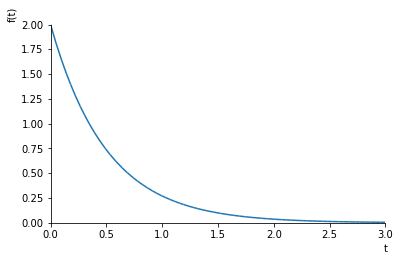
投稿日：2020-05-15T14:00:54+09:00

Python実装中に開発環境でよく使うコマンド

自分用メモですが。。。随時追加予定。

前提

プロジェクトルートに移動した状態で使う。

venv起動／停止

venv\script\activate
venv\script\deactivate

サーバー起動

python manage.py runserver --setting={prj_name}.local_settings.py

proxy認証

set HTTP_PROXY=http://{id}:{password}@{host}:{port}
set HTTPS_PROXY=http://{id}:{password}@{host}:{port}

　 Tweet
Qiitaで続きを読む

投稿日：2020-05-15T13:51:09+09:00

AtCoder Beginner Contest 107 過去問復習

所要時間

感想

D問題が難しくバチャコン後も2,3日の間格闘してました。
だいぶ考察力が必要かつBIT(BinaryIndexedTree)の知識も必要だったので、まとめていきたいと思います。BITについては別の記事で自分なりにわかりやすく説明したので参考にしてください。

A問題

出力すべきなのはn-i+1であることに注意してください。
answerA.py
n,i=map(int,input().split())
print(n-i+1)
B問題

こういうマス目の問題でnumpyを使いたいですね。
近いうちにnumpyの操作も学んでいけたらと思います。
行,列を除く操作を別々に行うと実装がわかりやすいです。
answerB.py
h,w=map(int,input().split())
a=[]
#白いマス目のみからなる行を除く
for i in range(h):
    k=input()
    if k!="."*w:
        a.append(k)
l=len(a)

ans=[[] for i in range(l)]
#白いマス目のみからなる列を除く
for i in range(w):
    for j in range(l):
        if a[j][i]=="#":
            for k in range(l):
                ans[k].append(a[k][i])
            break
for i in range(l):
    print("".join(ans[i]))
C問題

k本の連続するろうそくに火をつけるのが最適であり、その候補はn-k+1通りあります。さらに、初めは座標0の地点にいるので、座標0→左端→右端へと進むパターンと座標0→右端→左端へと進むパターンの二つがそれぞれの候補で存在するので、この$2 \times (n-k+1)$通りの中で最小の時間(=進む距離)を求めれば良いです。
answerC.py
n,k=map(int,input().split())
x=list(map(int,input().split()))
mi=10**10
for i in range(n-k+1):
    mi=min(mi,x[k-1+i]-x[i]+min(abs(x[i]),abs(x[k-1+i])))
print(mi)
D問題

中央値をうまく探そうとしたのですが、与えられる数列がそもそもソート済みなものだと誤読していました。
また、正答を読んで理解しましたが、かなり難しく実力不足であると感じました。しかし、かなりためになる問題であったので詳しく解説をしていきたいと思います。
また、先の感想でも述べたようにBITを既知のものとして解説をしますので、BITについいてはこの記事を参照してください。

まず、中央値の条件を求めやすいように抽象化する必要があります(この抽象化のセンスは問題を多く解くほど上がっていきそうです)。

長さMの数列bについて中央値がxであると仮定すれば、①:b中にx以上の要素は$[\frac{M}{2}]$以上存在し、②:①を満たす中でxは最大、という二条件が必要です。…(✳︎)

ここからわかるのは単調性を持つことです。したがって、中央値は二分探索で探すことができることがわかります(中央値→二分探索は頻出のようです。)。

二分探索で探せることがわかったので、以下では「題意の数列$m$の中央値がx以上になる条件」…(1)を考えていきます。

(✳︎)から、(1)は、$(a_l,a_{l+1},…,a_{r})$の中央値を$m_{l,r}(1 \leqq l \leqq r \leqq N)$とした時にx以上になる$m_{l,r}$が$[\frac{_{n+1} C _2}{2}]$個以上ある…(2)、と言い換えることができます。

さらに、同様に(✳︎)を用いれば、$m_{l,r}$がx以上になるには$(a_l,a_{l+1},…,a_{r})$にx以上の要素が$[\frac{r-l+1}{2}]$個以上あれば良いこともわかります。…(3)

したがって、x以上かx未満かという情報のみが必要なので、前者は1で後者は-1で置き換えてしまえば、(3)は、$(a_l,a_{l+1},…,a_{r})$の要素の累積和$S_{l,r}$が0以上…(4)、と言い換えることができます。

ここで、累積和により$(a_1,a_2,…,a_{k})$の累積和$S_k$を先に求めて保存しておけば、$S_{l,r}=S_r-S_{l-1}$であり、(4)は、$S_r-S_{l-1} \geqq 0 \leftrightarrow S_{l-1} \leqq
S_r$…(5)、と言い換えることができます。

さらに、(5)は、$S_{l-1} \leqq
S_r (1 \leqq l \leqq r \leqq N)$、であるので、$S_l \leqq S_r (0 \leqq l < r \leqq N)$…(6)、と言い換えても同値になります。

以上の考察より、(1)の条件は、$0 \leqq l < r \leqq N$を満たす$l,r$で$S_l \leqq S_r$となるものが$[\frac{_{n+1} C _2}{2}]$個以上ある、と言い換えることができ、これを求めることを考えます。

また、この時に$l,r$をそれぞれ考えると、計算量が$O(n^2)$になりますが、rを固定した(r*)もとで、$S_l \leqq S_{r^*}$かつ$0 \leqq l < r^*$を満たす$l$は実はBITを使って$O(\log{n})$で求められるので、$O(n \log{n})$で$l,r$の組を決定することができます。

先ほどのBITを使用する際には、BITで管理する配列$B$の$i$番目の要素(1-indexed)を、累積和$S_r(0 \leqq r \leqq r^*-1)$のうち$i$になるものが何回出てきたか、とすることで、$S_l \leqq S_{r^*}$かつ$0 \leqq l < r^*$を満たす$l$を$B_1+B_2+…+B_{S_{r^*}}$で求めることができます。

また、累積和$S_r(0 \leqq r \leqq r^*-1)$のうち$i$になるものが何回出てきたかについては、それぞれのrで$B_{S_{r}}$を加算すれば良いです。

さらに、累積和$S_r(0 \leqq r \leqq n)$は0以下になる可能性があるので、最小値が1になるように$1-S_min$を全ての累積和に足しています。

以上を全て実装すれば以下のようになります。

✳︎…実装方針が立った後もインデックスをミスってセグフォを出したり出力すべきものを間違えたりしたので気をつけていきたいです。
answerD.cc
//インクルード(アルファベット順,bits/stdc++.hは使わない派閥)
#include<algorithm>//sort,二分探索,など
#include<bitset>//固定長bit集合
#include<cmath>//pow,logなど
#include<complex>//複素数
#include<deque>//両端アクセスのキュー
#include<functional>//sortのgreater
#include<iomanip>//setprecision(浮動小数点の出力の誤差)
#include<iostream>//入出力
#include<iterator>//集合演算(積集合,和集合,差集合など)
#include<map>//map(辞書)
#include<numeric>//iota(整数列の生成),gcdとlcm(c++17)
#include<queue>//キュー
#include<set>//集合
#include<stack>//スタック
#include<string>//文字列
#include<unordered_map>//イテレータあるけど順序保持しないmap
#include<unordered_set>//イテレータあるけど順序保持しないset
#include<utility>//pair
#include<vector>//可変長配列

using namespace std;
typedef long long ll;

//マクロ
//forループ関係
//引数は、(ループ内変数,動く範囲)か(ループ内変数,始めの数,終わりの数)、のどちらか
//Dがついてないものはループ変数は1ずつインクリメントされ、Dがついてるものはループ変数は1ずつデクリメントされる
#define REP(i,n) for(ll i=0;i<(ll)(n);i++)
#define REPD(i,n) for(ll i=n-1;i>=0;i--)
#define FOR(i,a,b) for(ll i=a;i<=(ll)(b);i++)
#define FORD(i,a,b) for(ll i=a;i>=(ll)(b);i--)
//xにはvectorなどのコンテナ
#define ALL(x) (x).begin(),(x).end() //sortなどの引数を省略したい
#define SIZE(x) ((ll)(x).size()) //sizeをsize_tからllに直しておく
#define MAX(x) *max_element(ALL(x)) //最大値を求める
#define MIN(x) *min_element(ALL(x)) //最小値を求める
//定数
#define INF 1000000000000 //10^12:極めて大きい値,∞
#define MOD 1000000007 //10^9+7:合同式の法
#define MAXR 100000 //10^5:配列の最大のrange(素数列挙などで使用)
//略記
#define PB push_back //vectorヘの挿入
#define MP make_pair //pairのコンストラクタ
#define F first //pairの一つ目の要素
#define S second //pairの二つ目の要素


//1-indexed
class BIT {
public:
    ll n; //データの長さ
    vector<ll> bit; // データの格納先
    BIT(ll n):n(n),bit(n+1,0){} //コンストラクタ

    //bit_i にxをO(log(n))で加算する
    void add(ll i,ll x){
        if(i==0) return;
        for(ll k=i;k<=n;k+=(k & -k)){
            bit[k]+=x;
        }
    }

    //bit_1 + bit_2 + … + bit_n-1 + bit_n をO(log(n))で求める
    ll sum(ll i){
        ll s=0;
        if(i==0) return s;
        for(ll k=i;k>0;k-=(k & -k)){
            s+=bit[k];
        }
        return s;
    }
};

ll solve(vector<ll>& a,ll x,ll n){
    vector<ll> b(n,-1);
    REP(i,n)if(a[i]>=x)b[i]=1;
    vector<ll> s(n+1,0);

    //ここ違った…
    FOR(i,1,n)s[i]=s[i-1]+b[i-1];

    ll base=1-MIN(s);REP(i,n+1)s[i]+=base;
    BIT T(MAX(s));
    ll ret=0;
    REP(i,n+1){
        ret+=T.sum(s[i]);
        T.add(s[i],1);
    }
    return ret;
}

signed main(){
    ll n;cin >> n;
    vector<ll> a(n,0);vector<ll> c(n,0);
    REP(i,n){cin >> a[i];c[i]=a[i];}
    sort(ALL(c));c.erase(unique(ALL(c)),c.end());
    //答えを二分探索で探す
    ll check=((n+1)*n/2)/2;
    ll l,r;l=0;r=SIZE(c)-1;
    while(r>l+1){
        ll h=(l+r)/2;
        if(solve(a,c[h],n)>=check){
            l=h;
        }else{
            r=h;
        }
    }
    #if 0
    //デバッグ用コード
    REP(i,SIZE(c)){
        cout << c[i] << " " << solve(a,c[i],n) << endl;
    }
    #endif

    //ここでもlとrを反対にするミス…
    if(solve(a,c[r],n)>=check){
        cout << c[r] << endl;
    }else{
        cout << c[l] << endl;
    }
}

　 Tweet
Qiitaで続きを読む

投稿日：2020-05-15T13:20:27+09:00

XPath基礎編（1）ー XPathの基本概念

Webサイト上からデータを自動的に取得するには2つの方法があります。1つはPythonなどのプログラミング言語でWebクローラーを作る、もう1つはOctoparseのようなWebスクレイピングツールでデータを取得するのです。しかし、どれにしても、XPathは重要な役割を果たしています。XPathの書き方が分かれば、データをより正しくて効率的に取得できます。

それでXPathのシリーズではXPathの基本概念からXPathの書き方、応用まで詳しく紹介したいと思います。

この記事では、XPathの基本概念を簡単に紹介します。

1. XPathとは？

XPath (XML Path Language)とは、ツリー構造となっているXML/HTMLドキュメントからの要素や属性値などを指定するための簡潔な構文(言語)です。
Webページは通常HTMLで記述されるから、XPathはWebページの情報を取得する時によく利用します。ブラウザ（Chrome、Firefoxなど）でWebページのHTMLを表示するする場合、F12キーを押すことで、対応するHTMLドキュメントに簡単にアクセスできます。

2. XPathの仕組み

XPathは具体的にはどのように動作するのかを見てみましょう。下記の画像はHTMLドキュメントの一部です。

HTMLは、ツリー構造のように、異なるレベルのがあります。この例では、レベル1はbookstoreで、レベル2は
bookです。Title、author、year、priceはすべてレベル3です。

山括弧（など）を含むテキストはタグと呼ばれます。HTMLの要素は通常、開始タグと終了タグで構成され、その間にコンテンツが挿入されます。以下の形になります。

<○○>(開始タグ)ここにコンテンツが入ります... </○○>(終了タグ)

XPathはスラッシュ “/” で区切りながら階層を記述し、基準となるノードから別のノードを指定できます。URLと似ています。この例では、要素「author」を検索する場合、XPathは次のようになります。

/bookstore/book/author

それがどのように機能するかをよりよく理解するには、コンピューター上の特定のファイルを見つける方法を参照してください。

「author」という名前のファイルを見つけるには、正しいファイルパスは\ bookstore \ book \ authorです。

コンピューター上のすべてのファイルには独自のパスがあるように、Webページ上の要素もパスがあります。そのパスはXPathで記述されています。

ルート要素（ドキュメントの一番上の要素）から始まり、中にあるすべての要素を経由して目標要素に至るXPathは、絶対XPathと呼ばれます。

例：　/html/body/div/div/div/div/div/div/div/div/div/span/span/span…

絶対XPathは長くて混乱する可能性があるため、絶対XPathを単純化するために、「//」を使用して途中までのパスを省略することができます（短いXPathとも呼ばれる）。

たとえば、

絶対XPath：　　/bookstore/book/author
短いXPath：　　//author

3. XPathを表示・書くには

【Google Chromeの場合】

Chromeでこのページを表示し、右クリックメニューの[検証]から開発者ツールを表示します。Elementタブのhtmlで、要素を右クリックします。メニューの[Copy] → [Copy XPath ] でその要素を取得するためのXPathがクリップボードにコピーされます。

表示されているElementタブのhtmlから “Ctrl + F” で検索欄を表示します。XPathを入力すると、得られる要素が選択されるはずです。

また、「XPath Helper」という拡張機能を追加することもできます。XPathを入力すると、一致する結果が表示されます。（XPath Helperをインストールする)

【Firefoxの場合】　

Firefoxの旧バージョンに搭載されている拡張機能「Firebug」が利用できます。（Firebug&FireXPath拡張機能をインストールする方法)

FirefoxでWebページを開く➡Firebugボタンをクリック➡ページ内の要素をクリック➡その要素のXPathが表示されます。

以上はXPathの基本概念でした。次回はXPathの書き方を紹介しますので、お楽しみにしてください！

　 Tweet
Qiitaで続きを読む

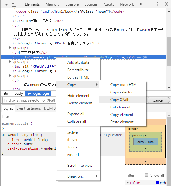
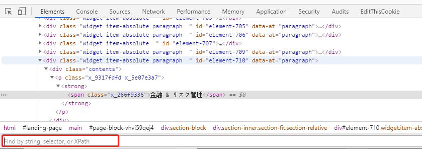
投稿日：2020-05-15T13:11:01+09:00

宇宙の研究を初める人向けのgoogle Colabで行うイメージ解析

はじめに

fits ファイルを扱うのが初めての人向けです．銀河の画像は親やすいので，これを例に google Colab だけでも動くサンプルです．もう少し上級者向けに書いた pythonのastroqueryを用いて検索し、skyviewでfits画像を取得する方法もあります．

基本編

サーバーとクライエントの基本

宇宙天文では，大量のデータをやりとりするので，サーバーとクライエント，について知識が必要になります．クライアントサーバ (client server system) とは，宇宙天文でも基本となるコンセプトなので，知っておこう．簡単には，サーバーとは，ネットワーク上のたくさんの機器に情報を提供できる機能が備わったOSやソフトウェア群のことで，クライエントはサーバーからデータを取得するだめのマシンのことです．

OSによってもかなり違いがあります．宇宙天文では，linuxベースのサーバがほぼ100%だと思いますので，基本的なサーバーとのやりとりや仕組みを事前に知っておくと，宇宙天文のデータを取得する際に少しは気が楽になると思います．サーバーOSとは？などを参考ください．

urllib の例

サーバーとクライエントの仕組みを使う場合は，今ではとても簡単なので，まずは気楽に使ってみよう．例えば，NASAのheasoftという有名なページのファイルを取得してみよう．
import urllib.request
from bs4 import BeautifulSoup
url = 'https://heasarc.gsfc.nasa.gov/docs/software/heasoft/'
req = urllib.request.Request(url)
html = urllib.request.urlopen(req)
soup = BeautifulSoup(html, "html.parser")
topicsindex = soup.find('div', attrs={'class': 'navigation'})
これで，soup に全htmlの情報が取得されている．ブラウザはこれを表示しているのである．この中から，navigation という部分だけ取得したのが，topicsindex であり，
print(topicsindex) # extract sentences begining with div navigation 
<div class="navigation">
<div id="nasaHeader">
<div>
....
のように，一部の情報だけ表示される．これは，クライエントからNASAのサーバーにアクセスし，データをもらうという作業で，数行のプログラムで書けることに注目してほしい．データを取得するというのは，ブラウザからマウスでボタンを色々と押してデータを取得する，というだけではないことを認識して欲しいのと，宇宙天文の場合はこのようなコマンドラインでデータを取得することが多い．

astroquery の設定
pip install astroquery 
で astroquery をインストールしよう．これはskyviewやvizierなど，多々のカタログから，同じコーディングでデータを取得するためのツールです．

vizier の使い方

vizierは論文ごとにカタログを抽出したものである．例えば，blackhole で検索すると，大量のカタログを含む論文のリストが現れる．vizier上でも簡単なプロットなどがすぐにできる．論文とも紐付けられているので，もと情報にもすぐに辿れるのも便利．astroquery からは，
# download galaxy data via Vizier
from astroquery.vizier import Vizier 
v = Vizier(catalog="J/ApJS/80/531/gxfluxes",columns=['Name',"logLx","Bmag","dist","type"],row_limit=-1)
data = v.query_constraints()
sname = data[0]["Name"] 
namelist = []
olist=["HRI","DSS"]
J/ApJS/80/531/gxfluxes は銀河のカタログで，ここから，'Name',"logLx","Bmag","dist","type" のデータを抽出して，sname = data[0]["Name"] として， Name だけ取り出している．

skyview の使い方

skyview は，天体の画像を取得するのに便利なカタログです．今回はここから銀河の画像を取得してみましょう．
# get image from skyview
from astroquery.skyview import SkyView
name=namelist[0]
paths = SkyView.get_images(position=name, survey=olist)
save(paths,name,olist)
ここでは，position="天体名", survey=["DSS",..]などを指定して，
skyview から画像を取得し，save という関数で fits ファイルに保存する．

fitsファイルへの保存方法
def save(p,name,obs): # save file into fits 
    for onep,oneo in zip(p,obs):
        onep.writeto(name+"_"+oneo+".fits",overwrite=True)
obs の中に書かれたカテゴリリストの名前をつけて，fits ファイルに保存する．

matplotlib を用いた天空座標でのプロット例

画像をプロットするのに，必要なモジュールをインポートする．
import matplotlib.pyplot as plt
from matplotlib.colors import LogNorm
from astropy.wcs import WCS
from astropy.io import fits
import glob 
import numpy as np
次に，fits ファイルを astropy で読んで，header から WCS 情報を引き出す．
# set IC342 imaga of DSS
dssname = "IC0342_DSS.fits"
dsshdu = fits.open(dssname)[0]
dsswcs = WCS(dsshdu.header)
dssdata = dsshdu.data
matplotlib でプロットする．
# plot image 
F = plt.figure(figsize=(8,8))
plt.subplot(111, projection=dsswcs)
plt.imshow(dssdata, origin='lower', norm=LogNorm())
plt.colorbar() 
このような絵が表示されれば成功です．

画像解析の例

画像の回転，転置，差分，など基本的な操作をして画像で遊んでみよう．
例えば，差分画像も簡単に表示できます．

fits ファイルとは，テキストで書かれた基礎情報と，バイナリで書かれたデータが合わさったファイル，というだけで，本当にそれだけなので，まずは苦手意識を持たずに扱おう．画像データは，openCV など，python にはたくさんのモジュールがあるので，まずはいろいろと遊んでみましょう．画像も，銀河でも波長が違えば見え方が違うし，超新星残骸，銀河団など，他の画像で遊んでみるのもよいです．画像の検索方法は，vizier でもよいですが，意外と欲しいものが見つからないこともあるので，適当にgoogleで検索した方が早いときもあります．．

google Colab での実行例

google Colab 上で実行するには，astroquery がデフォルトではインストールされてないので，astroquery の install が必要です．google Colab 上での実行例を参照ください．

また，fits ファイルを google drive 上に保存しないと，データは外に出せないので，必要ならgoogle drive をマウントして，そこに fits ファイルを書き出しましょう．

関連ページ

python の astroquery を用いた宇宙天文カタログの検索と銀河を用いた簡単なプロット方法

WCS座標でイメージをマージしpythonでプロットする方法

pythonを用いて銀経銀緯で複数のfits画像を並べてプロットする方法

　 Tweet
Qiitaで続きを読む

	Province/State	Country/Region	Lat	Long	...	4/22/20	4/23/20	4/24/20	4/25/20	4/26/20	4/27/20	4/28/20	4/29/20	4/30/20	5/1/20
0	NaN	Afghanistan	33.0000	65.0000	...	1176	1279	1351	1463	1531	1703	1828	1939	2171	2335
1	NaN	Albania	41.1533	20.1683	...	634	663	678	712	726	736	750	766	773	782
2	NaN	Algeria	28.0339	1.6596	...	2910	3007	3127	3256	3382	3517	3649	3848	4006	4154
3	NaN	Andorra	42.5063	1.5218	...	723	723	731	738	738	743	743	743	745	745
4	NaN	Angola	-11.2027	17.8739	...	25	25	25	25	26	27	27	27	27	30

	1/22/20	1/23/20	1/24/20	1/25/20	1/26/20	1/27/20	1/28/20	1/29/20	1/30/20	1/31/20	...	4/22/20	4/23/20	4/24/20	4/25/20	4/26/20	4/27/20	4/28/20	4/29/20	4/30/20	5/1/20
Country/Region
Afghanistan	0	0	0	0	0	0	0	0	0	0	...	1176	1279	1351	1463	1531	1703	1828	1939	2171	2335
Albania	0	0	0	0	0	0	0	0	0	0	...	634	663	678	712	726	736	750	766	773	782
Algeria	0	0	0	0	0	0	0	0	0	0	...	2910	3007	3127	3256	3382	3517	3649	3848	4006	4154
Andorra	0	0	0	0	0	0	0	0	0	0	...	723	723	731	738	738	743	743	743	745	745
Angola	0	0	0	0	0	0	0	0	0	0	...	25	25	25	25	26	27	27	27	27	30

Country/Region	Australia	...	Vietnam
1/22/20	0	...	0
1/23/20	0	...	2
1/24/20	0	...	2
1/25/20	0	...	2
1/26/20	4	...	2

Country/Region	Afghanistan	Albania	Algeria	Andorra	Angola	Antigua and Barbuda	Argentina	Armenia	Australia	Austria	...	United Kingdom	Uruguay	Uzbekistan	Venezuela	Vietnam	West Bank and Gaza	Yemen	Zambia	Zimbabwe
4/22/20	84	25	99	6	1	1	113	72	7	52	...	4466	8	38	3	0	8	0	4	0
4/23/20	103	29	97	0	0	0	291	50	10	77	...	4608	14	42	23	0	6	0	2	0
4/24/20	72	15	120	8	0	0	172	73	15	69	...	5394	6	46	7	2	4	0	8	1
4/25/20	112	34	129	7	0	0	173	81	17	77	...	4929	33	58	5	0	-142	0	0	2
4/26/20	68	14	126	0	1	0	112	69	20	77	...	4468	10	7	2	0	0	0	4	0
4/27/20	172	10	135	5	1	0	111	62	7	49	...	4311	14	35	4	0	0	0	0	1
4/28/20	125	14	132	0	0	0	124	59	23	83	...	4002	5	35	0	0	1	0	7	0
4/29/20	111	16	199	0	0	0	158	65	8	45	...	4091	5	63	2	0	1	5	2	0
4/30/20	232	7	158	2	0	0	143	134	14	50	...	6040	13	37	2	0	0	0	9	8
5/1/20	164	9	148	0	3	1	104	82	12	79	...	6204	5	47	2	0	9	1	3	0

Country/Region	Afghanistan	Albania	Algeria	Andorra	Angola	Antigua and Barbuda	Argentina	Armenia	Australia	Austria	...	United Kingdom	Uruguay	Uzbekistan	Venezuela	Vietnam	West Bank and Gaza	Yemen	Zambia	Zimbabwe
4/22/20	7.692308	4.105090	3.521878	0.836820	4.166667	4.347826	3.728143	5.139186	0.105342	0.349627	...	3.430845	1.495327	2.264601	1.052632	0.000000	1.716738	0.000000	5.714286	0.000000
4/23/20	8.758503	4.574132	3.333333	0.000000	0.000000	0.000000	9.255725	3.394433	0.150331	0.515913	...	3.422511	2.578269	2.447552	7.986111	0.000000	1.265823	0.000000	2.702703	0.000000
4/24/20	5.629398	2.262443	3.990688	1.106501	0.000000	0.000000	5.007278	4.793171	0.225158	0.459939	...	3.873720	1.077199	2.616610	2.250804	0.746269	0.833333	0.000000	10.526316	3.571429
4/25/20	8.290155	5.014749	4.125360	0.957592	0.000000	0.000000	4.796230	5.075188	0.254605	0.510915	...	3.407771	5.861456	3.215078	1.572327	0.000000	-29.338843	0.000000	0.000000	6.896552
4/26/20	4.647984	1.966292	3.869779	0.000000	4.000000	0.000000	2.962963	4.114490	0.298775	0.508318	...	2.987250	1.677852	0.375940	0.619195	0.000000	0.000000	0.000000	4.761905	0.000000
4/27/20	11.234487	1.377410	3.991721	0.677507	3.846154	0.000000	2.852004	3.550974	0.104260	0.321839	...	2.798678	2.310231	1.872659	1.230769	0.000000	0.000000	0.000000	0.000000	3.225806
4/28/20	7.339988	1.902174	3.753199	0.000000	0.000000	0.000000	3.097677	3.263274	0.342211	0.543407	...	2.527345	0.806452	1.838235	0.000000	0.000000	0.292398	0.000000	7.954545	0.000000
4/29/20	6.072210	2.133333	5.453549	0.000000	0.000000	0.000000	3.828447	3.481521	0.118624	0.293026	...	2.519864	0.800000	3.249097	0.607903	0.000000	0.291545	500.000000	2.105263	0.000000
4/30/20	11.964930	0.913838	4.106029	0.269179	0.000000	0.000000	3.337223	6.935818	0.207346	0.324633	...	3.628914	2.063492	1.848152	0.604230	0.000000	0.000000	0.000000	9.278351	25.000000
5/1/20	7.554123	1.164295	3.694458	0.000000	11.111111	4.166667	2.348690	3.969022	0.177357	0.511261	...	3.596918	0.777605	2.305051	0.600601	0.000000	2.616279	16.666667	2.830189	0.000000

Country/Region	Afghanistan	Albania	Algeria	Andorra	Angola	Antigua and Barbuda	Argentina	Armenia	Australia	Austria	...	United Kingdom	Uruguay	Uzbekistan	Venezuela	Vietnam	West Bank and Gaza	Western Sahara	Yemen	Zambia	Zimbabwe
4/22/20	7.064018	5.462185	2.920284	-5.276382	6.250000	-15.384615	3.718200	6.250000	-12.214551	-9.498681	...	3.270797	-1.895735	-4.258555	-1.265823	-13.461538	2.046036	0.000000	0.000000	12.500000	-4.347826
4/23/20	9.072165	0.000000	-4.524540	-6.366048	0.000000	0.000000	10.896226	2.941176	-6.836056	-9.750567	...	3.411790	-7.729469	-5.480540	12.179487	-2.222222	-3.759398	-83.333333	0.000000	0.000000	0.000000
4/24/20	5.860113	2.390438	4.738956	-1.699717	0.000000	-9.090909	4.423650	0.119048	-5.064935	-4.199569	...	3.743980	-4.712042	-1.260504	0.571429	13.636364	1.041667	0.000000	-100.000000	22.222222	4.545455
4/25/20	9.642857	9.727626	4.141104	2.017291	0.000000	0.000000	4.480652	0.594530	-15.321477	-5.994755	...	3.332975	16.483516	-2.382979	2.840909	-10.000000	-36.082474	0.000000	NaN	0.000000	8.695652
4/26/20	3.745928	2.127660	6.701031	0.000000	5.882353	0.000000	1.091618	4.609929	-11.954766	-4.304504	...	3.232666	1.886792	-6.538797	-1.657459	0.000000	3.629032	0.000000	NaN	-2.272727	0.000000
4/27/20	11.930926	-0.694444	5.383023	-10.169492	5.555556	0.000000	2.815272	5.197740	-3.669725	-1.582674	...	3.051680	1.388889	-6.343284	-0.561798	0.000000	0.000000	0.000000	NaN	0.000000	-8.000000
4/28/20	8.134642	1.048951	2.226588	-4.402516	0.000000	0.000000	3.450863	4.296455	-5.714286	-6.559458	...	2.318102	-1.369863	-6.474104	0.000000	6.666667	5.058366	0.000000	NaN	16.279070	0.000000
4/29/20	5.512322	-2.768166	9.032671	-8.552632	-5.263158	0.000000	4.387237	3.192585	-4.444444	-7.472826	...	2.386758	-6.018519	-4.472843	1.129944	0.000000	0.370370	0.000000	inf	-20.000000	0.000000
4/30/20	13.521819	-3.202847	4.406580	-15.467626	0.000000	0.000000	2.605071	10.279441	-1.585624	-4.013705	...	3.845988	2.955665	0.000000	-2.234637	6.250000	-1.845018	0.000000	-40.000000	20.000000	34.782609
5/1/20	5.955604	-3.308824	5.796286	-0.425532	-5.555556	-30.000000	2.064997	2.986425	-2.255639	-6.578276	...	3.750518	-6.220096	-3.567447	1.142857	0.000000	3.383459	0.000000	33.333333	-33.333333	0.000000

Country/Region	Afghanistan	Albania	Algeria	Andorra	Angola	Antigua and Barbuda	Argentina	Armenia	Australia	Austria	...	United Kingdom	Uruguay	Uzbekistan	Venezuela	Vietnam	West Bank and Gaza	Western Sahara	Yemen	Zambia	Zimbabwe
4/27/20	71.30	14.30	76.35	15.90	0.95	0.50	133.30	46.55	52.50	118.15	...	6654.15	10.95	50.20	8.85	2.25	12.85	0.05	0.00	2.15	1.15
4/28/20	77.10	14.45	78.05	15.20	0.95	0.50	137.90	48.55	49.50	110.40	...	6808.40	10.80	46.95	8.85	2.40	13.50	0.05	0.00	2.50	1.15
4/29/20	81.35	14.05	85.10	13.90	0.90	0.50	143.95	50.10	47.30	102.15	...	6970.90	10.15	44.85	8.95	2.40	13.55	0.05	0.25	2.00	1.15
4/30/20	92.35	13.60	88.85	11.75	0.90	0.50	147.70	55.25	46.55	98.05	...	7239.00	10.45	44.85	8.75	2.55	13.30	0.05	0.15	2.40	1.55
5/1/20	97.85	13.15	94.00	11.70	0.85	0.35	150.75	56.90	45.50	91.60	...	7510.50	9.80	43.25	8.85	2.55	13.75	0.05	0.20	1.60	1.55

20200515のPythonに関する記事は30件です。

SwiftでN次元行列演算ライブラリを作ってみた

はじめに

概要

宣言

型

Indexing

その他関数一覧

インストール

SwiftPM

CocoaPods

Performance

個人的に気に入っているところ

最後に

参考

SwiftでN次元行列演算ライブラリMatftを作ってみた

はじめに

概要

宣言

型

Indexing

その他関数一覧

インストール

SwiftPM

CocoaPods

Performance

個人的に気に入っているところ

最後に

参考

ゼロから始めるLeetCode Day26「94. Binary Tree Inorder Traversal」

概要

問題

解法

【数式なしの量子コンピュータ】 新視点セルオートマトンとグローバー ２回目 １、０ではない重ね合わせでの初期状態

2-1. q-camの構造とモジュール

2-2. 1,0ではない確率的初期状態（ry 又は rx 又は u3 ゲートで作る）

2-3. Blueqatの状態ベクトル表示からのベクトルと確率の抽出

2-4. Blueqatのベクトルと観測

第二回目のサマリー

SwitchBot温湿度計の値をRaspberryPiでロギング

はじめに

SwitchBotとは？

必要なもの

手順

①RaspberrypiとセンサのBluetooth接続確認

センサの認識確認

②センサの測定値をPythonで取得

bluepyでの認識確認

センサ値取得スクリプトの作成

メインスクリプトの作成

③PythonからGASのAPIを叩いてスプレッドシートにデータ書き込み

④スクリプトの定期実行

英語論文の文章をショートカットキー1回で整形してDeepL翻訳に突っ込む

方法

Pythonスクリプト

バッチファイル

ショートカットキー割り当て

終わりに

論文の文章をショートカットキー1回で整形してDeepL翻訳に突っ込む

方法

Pythonスクリプト

バッチファイル

ショートカットキー割り当て

終わりに

好きな芸能人のテレビ出演情報をLINEに通知する

目的

概要

番組情報取得

LINE

使ったコード

実行

参考

Pythonを使ってCovid-19(コロナ)のデータを分析しよう【初心者向け】

対象

本記事について

演習

Analyzing Coronavirus with Python (COVID-19) by NeuralNine on Youtube

直近10日(2020/04/22-05/01)の現在進行形の感染者数の増加率 (中国・イタリア・アメリカ・日本)

【強化学習】R2D2を実装/解説してみたリベンジ ハイパーパラメータ解説編（Keras-RL）

コード全体

【数式なしの量子コンピュータ】　新視点セルオートマトンとグローバー　　２回目１、０ではない重ね合わせでの初期状態

2-4.　Blueqatのベクトルと観測

【強化学習】R2D2を実装/解説してみたリベンジハイパーパラメータ解説編（Keras-RL）